Animating Channel Condition Number Along a UE Trajectory
This notebook demonstrates how to use NeoRadium to evaluate and animate the condition number of a trajectory-based channel as a UE moves along a trajectory in a DeepMIMO scenario.
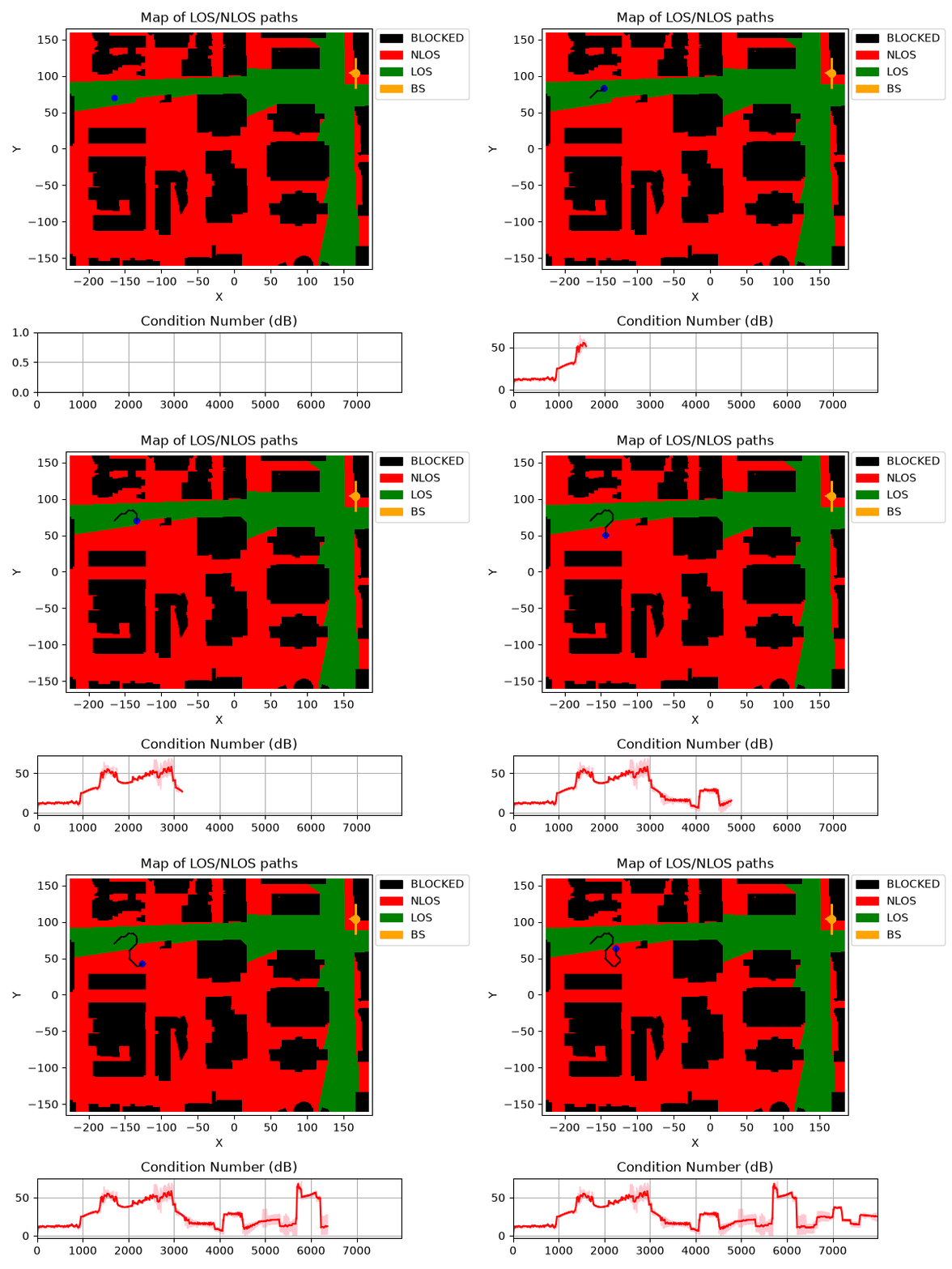
The notebook first opens a DeepMIMO scenario, creates a random UE trajectory, and then creates a TrjChannel object from that trajectory. As the UE moves along the trajectory, the notebook computes the channel condition number from the channel matrix and updates an animation.
The animation shows the UE moving along the trajectory on the DeepMIMO map. Below the map, two graphs are updated as the UE moves:
Condition number: shows the average condition number over each animation update interval, with a shaded region indicating the minimum-to-maximum range.
Number of paths: shows the average number of propagation paths over each animation update interval.
Notes
The condition number is computed from the channel matrix generated by the trajectory-based channel model.
The condition-number curve summarizes the channel over each animation update interval rather than showing every individual trajectory point.
The
trajLenparameter refers to the number of DeepMIMO grid points used for the trajectory, not the final number of interpolated trajectory points.The user may need to update the
dataFoldervariable based on the location of the DeepMIMO scenario files on their system.The generated animation is saved as a GIF file and then displayed in the notebook.
[1]:
import numpy as np
import matplotlib
from IPython.display import HTML, Markdown, display

from neoradium import DeepMimoData, TrjChannel, BandwidthPart, AntennaPanel, random
from neoradium.utils import toDb
[2]:
# Replace this with the folder on your system where the DeepMIMO scenarios are stored
dataFolder = "/data/RayTracing/DeepMIMO/Scenarios/V4/"
DeepMimoData.setScenariosPath(dataFolder)

# Create a DeepMimoData object
deepMimoData = DeepMimoData("asu_campus_3p5")
deepMimoData.print()
DeepMimoData Properties:
  Scenario:                   asu_campus_3p5
  Version:                    4.0.0a3
  UE Grid:                    rx_grid
  Grid Size:                  411 x 321
  Base Station:               BS (at [166. 104.  22.])
  Total Grid Points:          131,931
  UE Spacing:                 [1. 1.]
  UE bounds (xyMin, xyMax)    [-225.55 -160.17], [184.45 159.83]
  UE Height:                  1.50
  Carrier Frequency:          3.5 GHz
  Num. paths (Min, Avg, Max): 0, 6.21, 10
  Num. total blockage:        46,774
  LOS percentage:             19.71%
[3]:
random.setSeed(123)                                 # Make results reproducible
bwp = BandwidthPart(numRbs=24, spacing=15)          # Create a BandwidthPart object

# Create a random trajectory
trajectory = deepMimoData.getRandomTrajectory(xyBounds=np.array([[-210, 40], [-120, 100]]),   # Trajectory bounds
                                              segLen=5,     # Number of DeepMIMO grid points on the shortest segment
                                              bwp=bwp,      # The bandwidth part
                                              trajLen=100,  # Number of DeepMIMO grid points on the trajectory
                                              speedMps=15)  # Speed in m/s

trajectory.print()                                  # Print the trajectory information
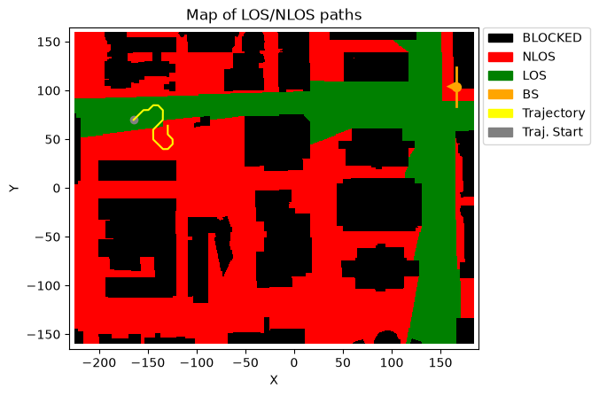
ax = deepMimoData.drawMap("LOS-NLOS", trajectory)   # Draw the map with the trajectory
deepMimoData.drawBsPanel(ax, 180)                   # TX antenna with a 180-degree bearing angle
Trajectory Properties:
  start (x,y,z):          (-164.55, 69.83, 1.50)
  No. of points:          7,984
  curIdx:                 0 (0.00%)
  curSpeed:               [10.64 10.64  0.  ]
  Total distance:         119.71 meters
  Total time:             7.983 seconds
  Average Speed:          14.996 m/s
  Carrier Frequency:      3.5 GHz
  Paths (Min, Avg, Max):  6, 8.90, 10
  Totally blocked:        0
  LOS percentage:         48.58%
[4]:
channel = TrjChannel(bwp, trajectory,
                     txOrientation = [180,0,0], # BS antenna facing the left side of the map
                     txAntenna = AntennaPanel([2,4]),  # 8 TX antennas
                     rxAntenna = AntennaPanel([1,2]),  # 2 RX antennas
                     seed = 123)
print(channel)

def getConditionNumber(channelMatrix):
    # Condition number:
    # CN(H) = 20 log10(sigmaMax/sigmaMin)
    # NOTE: CN is given on a logarithmic scale in dB. Values between 0 and
    # 10 dB are usually considered good for beamforming, while values above 20 dB
    # are considered unusable for beamforming.
    u, s, v = np.linalg.svd(channelMatrix)
    cn = 2 * toDb(s.max(axis=2) / np.maximum(s.min(axis=2), np.finfo(float).eps))
    return cn.min(), cn.mean(), cn.max()

# A callback function used to draw condition-number and path-count graphs below the animated trajectory
def handleGraph(request, ax, trajectory, points=None):
    if request=="Config":
        # Configure both graphs
        ax[0].set_xlim(0,trajectory.numPoints)
        ax[0].set_ylim(0, 70)
        ax[0].set_title("Condition Number (dB)")
        ax[0].grid()
        ax[0].plot([], [], 'red', markersize=1)
        ax[0].fill_between([], [], [], color='pink', alpha=0.5)

        if len(ax) > 1:  # Set `numGraphs` to 2 to draw the number of paths in the second graph
            ax[1].set_xlim(0,trajectory.numPoints)
            ax[0].set_ylim(0,30)
            ax[1].set_title("Number of Paths")
            ax[1].grid()
            ax[1].plot([], [], 'blue', markersize=1)

    elif request=="ConfigMap":
        # Customize the drawn map
        ax.drawBsPanel(180)         # Draw TX antenna panel (180-degree bearing angle)

    elif request=="Draw":
        # Per-frame updates to the graphs below the map
        # ax is an array with `numGraphs` elements
        p0, p1 = points
        cnMin, cnMean, cnMax, numPaths = [], [], [], []
        while channel.trajectory.curIdx < p1:
            cn = getConditionNumber( channel.getChannelMatrix() )
            cnMin += [cn[0]]
            cnMean += [cn[1]]
            cnMax += [cn[2]]
            numPaths += [channel.numPaths]
            channel.goNext()
        cnMin, cnMean, cnMax, numPaths = min(cnMin), np.mean(cnMean), max(cnMax), np.mean(numPaths)

        updatedItems = (ax[0].addNewPoint(p1, cnMean),
                        ax[0].addNewRange(p1, cnMin, cnMax) )
        if len(ax) > 1:  # Set `numGraphs` to 2 to draw the number of paths in the second graph
            updatedItems += (ax[1].addNewPoint(p1, numPaths),)
        print(f"\rProcessed trajectory point: {p1}", end="")
        return updatedItems
TrjChannel Properties:
  carrierFreq:              3.5 GHz
  normalizeGains:           True
  normalizeOutput:          True
  normalizeDelays:          True
  xPolPower:                10.00 (dB)
  filterLen:                16 samples
  delayQuantSize:           64
  stopBandAtten:            80 dB
  dopplerShift:             175.6 Hz
  coherenceTime:            2.409 milliseconds
  TX Antenna:
    Total Elements:         8
    spacing:                0.5𝜆, 0.5𝜆
    shape:                  2 rows x 4 columns
    polarization:           |
    Orientation (𝛼,𝛃,𝛄):     180° 0° 0°
  RX Antenna:
    Total Elements:         2
    spacing:                0.5𝜆, 0.5𝜆
    shape:                  1 rows x 2 columns
    polarization:           |
  Trajectory:
    start (x,y,z):          (-164.55, 69.83, 1.50)
    No. of points:          7,984
    curIdx:                 0 (0.00%)
    curSpeed:               [10.64 10.64  0.  ]
    Total distance:         119.71 meters
    Total time:             7.983 seconds
    Average Speed:          14.996 m/s
    Carrier Frequency:      3.5 GHz
    Paths (Min, Avg, Max):  6, 8.90, 10
    Totally blocked:        0
    LOS percentage:         48.58%
[5]:
# Create the animation, save it as a GIF, and display it below. This step may take some time.
channel.restart()
anim = deepMimoData.animateTrajectory(trajectory, numGraphs=1, pointsPerFrame=20,
graphCallback=handleGraph, fileName='AnimateCN.gif')
display(Markdown(""))
# Another option is to use the following command which gives you more controls for running
# the animation.
# # Increase the animation memory limit for HTML-based animation display
# matplotlib.rcParams['animation.embed_limit'] = 100000000
# HTML(anim.to_jshtml())
Processed trajectory point: 7960
[ ]: