End-to-End PDSCH Simulation with a Trajectory-Based Channel Model
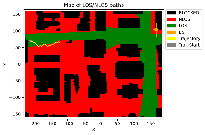
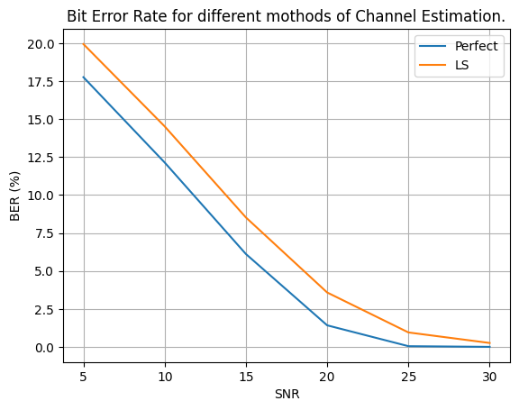
This notebook demonstrates how to use NeoRadium with a DeepMIMO ray-tracing scenario to simulate an end-to-end 5G NR PDSCH link while the UE moves along a trajectory. The example starts by opening a DeepMIMO scenario, selecting a base station and user grid, and creating a random trajectory through the DeepMIMO user grid. The trajectory-based channel model is then used in a slot-by-slot PDSCH simulation to measure the bit error rate (BER) at different SNR values.
The main goal is to compare two receiver-side channel estimation assumptions:
Perfect channel knowledge: the receiver uses the exact effective channel.
LS + interpolation: the receiver estimates the channel from the received grid using least-squares estimation and interpolation.
For simplicity, both cases use the same perfect-channel precoder at the transmitter. This keeps the example focused on the receiver-side channel estimation difference and avoids adding extra complications related to transmitter-side CSI acquisition or precoder estimation.
A few implementation notes:
The
dataFoldervariable should point to the folder where the DeepMIMO scenario files are stored on your system. Update it if your local DeepMIMO data is in a different location.The
trajLenparameter used when generating the random trajectory refers to the number of DeepMIMO grid points used for the path. This is different from the number of trajectory points used by the channel model, since the trajectory points are obtained by interpolation between DeepMIMO grid points.The simulation uses only the first 5,000 trajectory points. This keeps the runtime manageable while still allowing the UE to move through a meaningful portion of the generated trajectory.
The final result is a BER-vs-SNR comparison for the two channel estimation methods.
[1]:
import numpy as np
import scipy.io
import time
import matplotlib.pyplot as plt

from neoradium import DeepMimoData, TrjChannel, BandwidthPart, PDSCH, AntennaPanel, random
[2]:
# Replace this with the folder on your system where the DeepMIMO scenarios are stored
dataFolder = "/data/RayTracing/DeepMIMO/Scenarios/V4/"
DeepMimoData.setScenariosPath(dataFolder)

# Create a DeepMimoData object
deepMimoData = DeepMimoData("asu_campus_3p5")
deepMimoData.print()
DeepMimoData Properties:
  Scenario:                   asu_campus_3p5
  Version:                    4.0.0a3
  UE Grid:                    rx_grid
  Grid Size:                  411 x 321
  Base Station:               BS (at [166. 104.  22.])
  Total Grid Points:          131,931
  UE Spacing:                 [1. 1.]
  UE bounds (xyMin, xyMax)    [-225.55 -160.17], [184.45 159.83]
  UE Height:                  1.50
  Carrier Frequency:          3.5 GHz
  Num. paths (Min, Avg, Max): 0, 6.21, 10
  Num. total blockage:        46,774
  LOS percentage:             19.71%
[3]:
random.setSeed(123)                                 # Make results reproducible
bwp = BandwidthPart(numRbs=24, spacing=15)          # Create the BandwidthPart object

# Create a random trajectory
trajectory = deepMimoData.getRandomTrajectory(xyBounds=np.array([[-210, 40], [-120, 100]]),   # Trajectory bounds
                                              segLen=2,     # Number of DeepMIMO grid points on the shortest segment
                                              bwp=bwp,      # The bandwidth part
                                              trajLen=100,  # Number of DeepMIMO grid points on the trajectory
                                              speedMps=14,  # Speed in m/s
                                              trajDir="+X") # Trajectory direction

trajectory.print()                                  # Print the trajectory information
ax = deepMimoData.drawMap("LOS-NLOS", trajectory)   # Draw the map with the trajectory
deepMimoData.drawBsPanel(ax, 180)                   # TX antenna at a 180-degree bearing angle
Trajectory Properties:
  start (x,y,z):          (-209.55, 69.83, 1.50)
  No. of points:          7,648
  curIdx:                 0 (0.00%)
  curSpeed:               [ 9.9 -9.9  0. ]
  Total distance:         107.30 meters
  Total time:             7.647 seconds
  Average Speed:          14.031 m/s
  Carrier Frequency:      3.5 GHz
  Paths (Min, Avg, Max):  6, 8.99, 10
  Totally blocked:        0
  LOS percentage:         29.11%
[4]:
numSlots = 5000                 # Number of OFDM slots; uses the first 5,000 trajectory points
snrDbs = [5,10,15,20,25,30]     # SNR values, in dB
freqDomain = True               # Set to False to apply the channel in the time domain

# Create a PDSCH object
pdsch = PDSCH(bwp, numLayers=2, modulation="16QAM")     # PDSCH with 2 layers
pdsch.setDMRS(configType=2, additionalPos=2)            # DMRS configuration
results = {}                                            # Store simulation results

# Create a trajectory-based channel model
channel = TrjChannel(bwp, trajectory,
                     txAntenna = AntennaPanel([2,4]),   # 8 TX antennas
                     txOrientation = [180,0,0],         # BS antenna facing the left side of the map
                     rxAntenna = AntennaPanel([1,2]),   # 2 RX antennas
                     seed = 123)

for chanEstMethod in ["Perfect", "LS"]:                 # Two channel estimation methods
    results[chanEstMethod] = {}
    print(f"\nRunning the end-to-end simulation with \"{chanEstMethod}\" channel estimation "
          f"in the {'frequency' if freqDomain else 'time'} domain.")
    print("SNR(dB)    Total Bits    Bit Errors   BER(%)   Point   time(sec.)")
    print("-------   ------------   ----------   ------   -----   ----------")
    for snrDb in snrDbs:
        random.setSeed(123)                             # Make the results reproducible
        t0 = time.monotonic()
        channel.restart()

        bitErrors = 0
        totalBits = 0

        for slotNo in range(numSlots):
            pdsch.initGrid()                            # Create a resource grid populated with DMRS
            numBits = pdsch.getBitCapacity()[0]         # Actual number of bits available in the resource grid
            txBits = random.bits(numBits)               # Create random binary data

            # Populate the resource grid with data, including QAM modulation and resource mapping.
            pdsch.setPdschData(txBits)

            channelMatrix = channel.getChannelMatrix()              # Get the channel matrix
            precoder = pdsch.getPrecodingMatrix(channelMatrix)      # Get the precoder matrix from the PDSCH object

            txGrid = bwp.createGrid(channel.txAntenna.numEl)        # Create the transmitted resource grid
            pdsch.precodeTo(txGrid, precoder)                       # Perform the precoding

            if freqDomain:
                rxGrid = txGrid.applyChannel(channelMatrix)         # Apply the channel in the frequency domain
                rxGrid = rxGrid.addNoise(snrDb=snrDb)               # Add noise
            else:
                txWaveform = txGrid.ofdmModulate()                  # OFDM modulation
                maxDelay = channel.getMaxDelay()                    # Get the maximum channel delay
                txWaveform = txWaveform.pad(maxDelay)               # Pad with zeros
                rxWaveform = channel.applyToSignal(txWaveform)      # Apply channel in time domain
                noisyRxWaveform = rxWaveform.addNoise(snrDb=snrDb, bwp=bwp)     # Add noise
                offset = channel.getTimingOffset()                  # Get the timing offset for synchronization
                syncedWaveform = noisyRxWaveform.sync(offset)       # Synchronization
                rxGrid = syncedWaveform.ofdmDemodulate(bwp)         # OFDM demodulation

            errVar = None
            if chanEstMethod == "Perfect":                          # Perfect channel knowledge
                estChannelMatrix = TrjChannel.getEffChannel(channelMatrix, precoder)
            else:                                                   # LS + interpolation channel estimation
                estChannelMatrix, errVar = pdsch.estimateChannel(rxGrid)

            eqGrid, llrScales = pdsch.equalize(rxGrid, estChannelMatrix, errVar)    # Equalization
            rxBits = pdsch.getHardBits(eqGrid)[0]                   # Demodulation (hard decision)
            bitErrors += np.abs(rxBits-txBits).sum()                # Calculate the number of bit errors
            totalBits += numBits
            print(f"{snrDb:^7d}   {totalBits:<12,d}   {bitErrors:<10,d}   {bitErrors*100/totalBits:^6.3f}"
                  f"   {slotNo+1:^5,d}   {time.monotonic()-t0:^10.2f}", end='\r')
            channel.goNext()                                        # Prepare the channel model for the next slot

        dt = time.monotonic()-t0                                    # Total time for this SNR
        results[chanEstMethod][snrDb] = {"totalBits":totalBits,
                                         "bitErrors":bitErrors,
                                         "BER":      bitErrors*100/totalBits,  # BER percentage
                                         "Time":     dt}
        print()

# Plot the results
for i,chanEstMethod in enumerate(['Perfect', 'LS']):
    bers = [results[chanEstMethod][snrDb]["BER"] for snrDb in snrDbs]
    plt.plot(snrDbs, bers, label=chanEstMethod)
plt.legend()
plt.title(f"Bit Error Rate for Different Channel-Estimation Methods\n"
          f"along the first {numSlots:,} trajectory points")
plt.grid()
plt.xlabel("SNR (dB)")
plt.xticks(snrDbs)
plt.ylabel("BER (%)")
plt.show()
Running the end-to-end simulation with "Perfect" channel estimation in the frequency domain.
SNR(dB)    Total Bits    Bit Errors   BER(%)   Point   time(sec.)
-------   ------------   ----------   ------   -----   ----------
   5      149,760,000    22,902,539   15.293   5,000     234.99
  10      149,760,000    15,291,978   10.211   5,000     234.88
  15      149,760,000    9,124,849    6.093    5,000     235.19
  20      149,760,000    5,234,897    3.496    5,000     235.25
  25      149,760,000    3,714,488    2.480    5,000     237.60
  30      149,760,000    3,029,572    2.023    5,000     234.70

Running the end-to-end simulation with "LS" channel estimation in the frequency domain.
SNR(dB)    Total Bits    Bit Errors   BER(%)   Point   time(sec.)
-------   ------------   ----------   ------   -----   ----------
   5      149,760,000    27,055,580   18.066   5,000     242.67
  10      149,760,000    18,667,701   12.465   5,000     240.65
  15      149,760,000    11,489,101   7.672    5,000     238.97
  20      149,760,000    6,697,518    4.472    5,000     237.22
  25      149,760,000    4,311,994    2.879    5,000     235.84
  30      149,760,000    3,376,237    2.254    5,000     234.05
[ ]: