Training A ResNet model for Channel Estimation
Now that we have a channel estimation dataset, we can train a model to receive the channel estimates at the pilot locations and predict the channel estimates for the whole channel matrix.
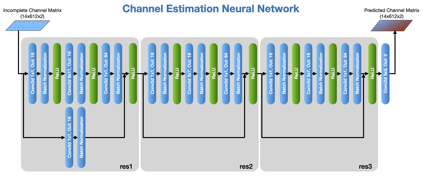
We use PyTorch freamework to train our models but other machine learning tools can also be used. The following diagram shows the Neural Network structure used for the channel estimation model.
So let’s get started by importing the required modules.
[1]:
import numpy as np
import time, datetime

import torch
from torch import nn
from torch.utils.data import Dataset, DataLoader
from torch.optim.lr_scheduler import ExponentialLR
Loading dataset
We first load our dataset files generated in the previous step. Then we create three sets of datasets and dataloaders for training, validation, and test.
[2]:
# Define our dataset object
class ChEstDataset(Dataset):
    def __init__(self, fileName):
        samples, labels = np.load(fileName)
        self.samples = np.float32(np.transpose(samples,(0,3,1,2)))
        self.labels = np.float32(np.transpose(labels,(0,3,1,2)))
        self.numSamples = len(self.samples)

    def __len__(self):
        return self.numSamples

    def __getitem__(self, idx):
        return self.samples[idx], self.labels[idx]

# Instantiate 3 datasets for train, validation, and test
trainDs = ChEstDataset("ChestTrain.npy")
validDs = ChEstDataset("ChestValid.npy")
testDs  = ChEstDataset("ChestTest.npy")

print(f"{len(trainDs)} Training Samples")
print(f"{len(validDs)} Validation Samples")
print(f"{len(testDs)} Test Samples")

# Create the data loaders
batchSize = 64
trainDl = DataLoader(trainDs, batchSize, shuffle=True)
validDl = DataLoader(validDs, batchSize, shuffle=False)
testDl = DataLoader(testDs, batchSize, shuffle=False)
16000 Training Samples
2400 Validation Samples
2400 Test Samples
[3]:
# Checking GPU availability
device = "cuda" if torch.cuda.is_available() else "mps" if torch.backends.mps.is_available() else "cpu"
print(f"Using {device} device")
Using cuda device
Creating the model
Now we can create a model object that will be used for training. We first define the ResBlock (See the picture above)
[4]:
# Define ResNet block
class ResBlock(nn.Module):
    def __init__(self, inDepth, midDepth, outDepth, kernel=(3,3), stride=(1,1)):
        super().__init__()
        if isinstance(stride, int): stride = (stride, stride)
        if isinstance(kernel, int): kernel = (kernel, kernel)

        self.conv1 = nn.Conv2d(inDepth, midDepth, 1, stride, padding='valid')  # 1x1 conv.
        self.bn1 = nn.BatchNorm2d(midDepth)
        self.conv2 = nn.Conv2d(midDepth, midDepth, kernel, padding='same')
        self.bn2 = nn.BatchNorm2d(midDepth)
        self.conv3 = nn.Conv2d(midDepth, outDepth, 1, stride, padding='valid') # 1x1 conv.
        self.bn3 = nn.BatchNorm2d(outDepth)
        self.relu = nn.ReLU(inplace=True)

        self.downSampleNet = None
        if ((stride != (1,1)) or (inDepth!=outDepth)):
            self.downSampleNet = nn.Sequential(nn.Conv2d(inDepth, outDepth, 1, stride),  # 1x1 conv.
                                               nn.BatchNorm2d(outDepth) )

        for bn in [self.bn1, self.bn2, self.bn3]:
            nn.init.ones_(bn.weight)
            nn.init.zeros_(bn.bias)

        for conv in [self.conv1, self.conv2, self.conv3]:
            nn.init.trunc_normal_(conv.weight, std=1/np.sqrt(np.prod(list(conv.weight.shape)[1:])))
            nn.init.zeros_(conv.bias)

        nn.init.zeros_(self.bn3.weight)  # This could improve results. It makes the block start like identity.

    def forward(self, x):
        out = self.conv1(x)
        out = self.bn1(out)
        out = self.relu(out)

        out = self.conv2(out)
        out = self.bn2(out)
        out = self.relu(out)

        out = self.conv3(out)
        out = self.bn3(out)

        if self.downSampleNet is None:  out += x
        else:                           out += self.downSampleNet(x)
        out = self.relu(out)

        return out
And now we define our Channel Estimator model (ChEstNet) using 2 instances of ResBlock defined above together with an additional convolutional layer.
[5]:
# Now the actual ChEstNet model
class ChEstNet(nn.Module):
    def __init__(self):
        super().__init__()
        self.res1 = ResBlock(2, 16, 64, (9,11))   # Res Block 9x11 kernel
        self.res2 = ResBlock(64, 16, 64, (3,7))   # Res Block 3x7 kernel
        self.res3 = ResBlock(64, 16, 64, (3,7))   # Res Block 3x7 kernel

        self.conv = nn.Conv2d(64, 2, 3, padding='same')
        nn.init.trunc_normal_(self.conv.weight, std=1/np.sqrt(np.prod(list(self.conv.weight.shape)[1:])))
        nn.init.zeros_(self.conv.bias)

    def forward(self, x):
        out = self.res1(x)
        out = self.res2(out)
        out = self.res3(out)
        out = self.conv(out)
        return out

# Instantiate the model and move it the target device
model = ChEstNet().to(device)
Training the model
Now we first create functions for the training and evaluation loops and use them to train the model.
Note: The following cell can take several hours to complete. A file containing the trained parameters of the model is included in this directory, so you can skip the following cells and proceed to the next step.
[6]:
# Training loop for one epoch:
def trainEpoch(dataLoader, model, lossFunction, optimizer):
    modelDevice = next(model.parameters()).device
    model.train() # Set the model to training mode
    lossMin, lossMean, lossMax = np.inf, 0, -np.inf
    for batchNo, (batchSamples, batchLabels) in enumerate(dataLoader):
        # Compute prediction and loss
        batchPredictions = model( batchSamples.to(modelDevice) )
        loss = lossFunction(batchPredictions, batchLabels.to(modelDevice))

        loss.backward()  # Backpropagation
        optimizer.step()
        optimizer.zero_grad()

        lossValue = loss.item()
        lossMean += lossValue
        if lossValue>lossMax: lossMax = lossValue
        if lossValue<lossMin: lossMin = lossValue

    lossMean /= len(dataLoader)
    return lossMin, lossMean, lossMax

# Evaluation loop:
def evaluate(dataLoader, model, lossFunction):
    modelDevice = next(model.parameters()).device
    model.eval()  # Set the model to evaluation mode
    numBatches = len(dataLoader)
    lossMean = 0

    with torch.no_grad():
        for batchNo, (batchSamples, batchLabels) in enumerate(dataLoader):
            batchPredictions = model( batchSamples.to(modelDevice) )
            lossMean += lossFunction(batchPredictions, batchLabels.to(modelDevice)).item()

    lossMean /= numBatches
    return lossMean

numEpochs = 100                    # Number of epochs
learningRate = (0.0001, 0.000001)  # Learning rate starts at 0.0001 and exponentially decays to 0.000001
lossFunction = nn.MSELoss()        # Using MSE as Loss

if isinstance(learningRate,tuple):  # learningRate is a tuple -> use exponentially decaying learning rate
    from torch.optim.lr_scheduler import ExponentialLR
    lr1st, lrLast = learningRate
    optimizer = torch.optim.Adam(model.parameters(), lr=lr1st)
    lrScheduler = ExponentialLR(optimizer, np.exp(np.log(lrLast/lr1st)/(numEpochs-1)))
else:
    optimizer = torch.optim.Adam(model.parameters(), lr=learningRate)  # learningRate is a number
    lrScheduler = None                                                 # No LR scheduling needed

t0 = time.time()
print("Epoch   Learning Rate   Training Loss   Validation Loss")
print("-----   -------------   -------------   ---------------")
lowestLoss = None
for epoch in range(numEpochs):
    print(" %-4d     %-10f      "%(epoch+1, lrScheduler.get_last_lr()[0]), end="")
    lossMin, lossMean, lossMax = trainEpoch(trainDl, model, lossFunction, optimizer)
    print("%-10f      "%(lossMean), end="")
    validLoss = evaluate(validDl, model, lossFunction)
    if lowestLoss is None:
        lowestLoss = validLoss
        print("%-10f   "%(validLoss))
    elif validLoss<lowestLoss:          # This is the best model so far -> Save it
        lowestLoss, bestEpoch = validLoss, epoch+1
        torch.save(model.state_dict(), 'Models/ChEstModelWeights.pth')
        print("%-10f * "%(validLoss))   # The '*' indicates best so far and saving
    else:
        print("%-10f   "%(validLoss))

    if lrScheduler is not None: lrScheduler.step()

print("Training complete. (Training Time: %s)"%(str(datetime.timedelta(seconds=int(time.time()-t0)))))
Epoch   Learning Rate   Training Loss   Validation Loss
-----   -------------   -------------   ---------------
 1        0.000100        0.099336        0.010627
 2        0.000095        0.005880        0.004009   *
 3        0.000091        0.003341        0.003787   *
 4        0.000087        0.002642        0.003150   *
 5        0.000083        0.002353        0.002327   *
 6        0.000079        0.002188        0.003565
 7        0.000076        0.002081        0.002741
 8        0.000072        0.001991        0.002619
 9        0.000069        0.001922        0.006631
 10       0.000066        0.001875        0.001991   *
 11       0.000063        0.001824        0.005979
 12       0.000060        0.001783        0.002245
 13       0.000057        0.001759        0.002502
 14       0.000055        0.001732        0.005101
 15       0.000052        0.001710        0.006416
 16       0.000050        0.001689        0.007298
 17       0.000048        0.001672        0.002904
 18       0.000045        0.001651        0.002459
 19       0.000043        0.001642        0.001740   *
 20       0.000041        0.001626        0.003589
 21       0.000039        0.001617        0.005713
 22       0.000038        0.001604        0.001715   *
 23       0.000036        0.001600        0.008538
 24       0.000034        0.001587        0.002987
 25       0.000033        0.001580        0.001638   *
 26       0.000031        0.001572        0.001692
 27       0.000030        0.001561        0.007471
 28       0.000028        0.001556        0.002036
 29       0.000027        0.001553        0.001821
 30       0.000026        0.001550        0.009173
 31       0.000025        0.001543        0.001734
 32       0.000024        0.001539        0.001667
 33       0.000023        0.001532        0.002818
 34       0.000022        0.001528        0.001524   *
 35       0.000021        0.001524        0.002134
 36       0.000020        0.001523        0.003879
 37       0.000019        0.001518        0.004665
 38       0.000018        0.001515        0.002332
 39       0.000017        0.001511        0.001507   *
 40       0.000016        0.001508        0.002086
 41       0.000016        0.001507        0.001654
 42       0.000015        0.001502        0.004450
 43       0.000014        0.001501        0.001833
 44       0.000014        0.001501        0.001561
 45       0.000013        0.001495        0.002375
 46       0.000012        0.001497        0.001502   *
 47       0.000012        0.001492        0.001637
 48       0.000011        0.001494        0.001482   *
 49       0.000011        0.001489        0.001800
 50       0.000010        0.001487        0.001888
 51       0.000010        0.001485        0.001501
 52       0.000009        0.001484        0.002236
 53       0.000009        0.001481        0.002009
 54       0.000008        0.001482        0.001516
 55       0.000008        0.001483        0.001748
 56       0.000008        0.001479        0.001698
 57       0.000007        0.001476        0.001729
 58       0.000007        0.001482        0.001572
 59       0.000007        0.001477        0.001511
 60       0.000006        0.001474        0.001515
 61       0.000006        0.001475        0.001533
 62       0.000006        0.001471        0.001487
 63       0.000006        0.001471        0.001529
 64       0.000005        0.001473        0.001546
 65       0.000005        0.001476        0.001488
 66       0.000005        0.001472        0.001477   *
 67       0.000005        0.001467        0.001483
 68       0.000004        0.001470        0.001610
 69       0.000004        0.001470        0.001461   *
 70       0.000004        0.001467        0.001480
 71       0.000004        0.001466        0.001468
 72       0.000004        0.001465        0.001454   *
 73       0.000004        0.001465        0.001468
 74       0.000003        0.001465        0.001503
 75       0.000003        0.001464        0.001458
 76       0.000003        0.001463        0.001510
 77       0.000003        0.001465        0.001461
 78       0.000003        0.001462        0.001459
 79       0.000003        0.001463        0.001452   *
 80       0.000003        0.001464        0.001558
 81       0.000002        0.001462        0.001476
 82       0.000002        0.001463        0.001454
 83       0.000002        0.001462        0.001475
 84       0.000002        0.001460        0.001508
 85       0.000002        0.001463        0.001491
 86       0.000002        0.001462        0.001494
 87       0.000002        0.001460        0.001454
 88       0.000002        0.001458        0.001521
 89       0.000002        0.001461        0.001483
 90       0.000002        0.001462        0.001453
 91       0.000002        0.001459        0.001519
 92       0.000001        0.001455        0.001471
 93       0.000001        0.001460        0.001474
 94       0.000001        0.001461        0.001458
 95       0.000001        0.001462        0.001468
 96       0.000001        0.001457        0.001454
 97       0.000001        0.001459        0.001464
 98       0.000001        0.001459        0.001469
 99       0.000001        0.001461        0.001459
 100      0.000001        0.001458        0.001489
Training complete. (Training Time: 0:51:55)
Evaluating the model
[7]:
testLoss = evaluate(testDl, model, lossFunction)
print(f"Test Loss: %.6f"%(testLoss))
Test Loss: 0.001446
[ ]: