Evaluating the Trained Channel Estimator
Now that we have a trained model, we can use it in the communication pipeline and compare its performance with baselines. In this case we compare it with perfect channel estimation and NeoRadium’s Least-Square channel estimation method.
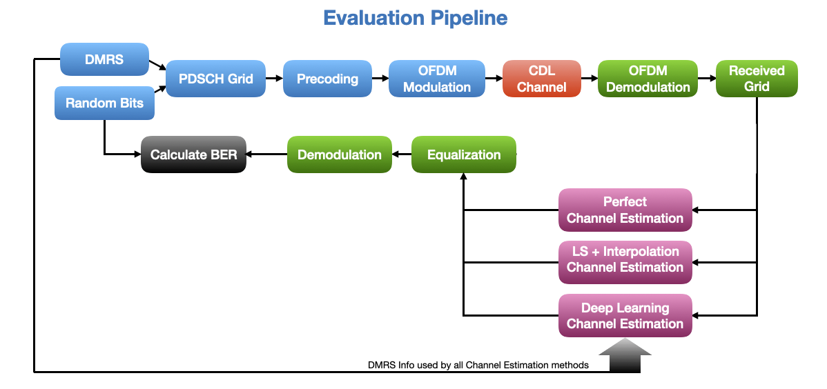
The following diagram shows the pipeline used for evaluation of our deep-learning-based channel estimator.
So, lets get started by importing the required modules.
[1]:
import numpy as np
import scipy.io
import time
import matplotlib.pyplot as plt

from neoradium import Carrier, PDSCH, CdlChannel, AntennaPanel, Grid, random

import torch
from torch import nn
Load the trained model
Here we define the channel estimator model and initialize it with the trained parameters.
[2]:
# ResNet Block
class ResBlock(nn.Module):
    def __init__(self, inDepth, midDepth, outDepth, kernel=(3,3), stride=(1,1)):
        super().__init__()
        if isinstance(stride, int): stride = (stride, stride)
        if isinstance(kernel, int): kernel = (kernel, kernel)

        self.conv1 = nn.Conv2d(inDepth, midDepth, 1, stride, padding='valid')  # 1x1 conv.
        self.bn1 = nn.BatchNorm2d(midDepth)
        self.conv2 = nn.Conv2d(midDepth, midDepth, kernel, padding='same')
        self.bn2 = nn.BatchNorm2d(midDepth)
        self.conv3 = nn.Conv2d(midDepth, outDepth, 1, stride, padding='valid') # 1x1 conv.
        self.bn3 = nn.BatchNorm2d(outDepth)
        self.relu = nn.ReLU(inplace=True)

        self.downSampleNet = None
        if ((stride != (1,1)) or (inDepth!=outDepth)):
            self.downSampleNet = nn.Sequential(nn.Conv2d(inDepth, outDepth, 1, stride),  # 1x1 conv.
                                               nn.BatchNorm2d(outDepth) )

        for bn in [self.bn1, self.bn2, self.bn3]:
            nn.init.ones_(bn.weight)
            nn.init.zeros_(bn.bias)

        for conv in [self.conv1, self.conv2, self.conv3]:
            nn.init.trunc_normal_(conv.weight, std=1/np.sqrt(np.prod(list(conv.weight.shape)[1:])))
            nn.init.zeros_(conv.bias)

        nn.init.zeros_(self.bn3.weight)  # This could improve results. It makes the block start like identity.

    def forward(self, x):
        out = self.conv1(x)
        out = self.bn1(out)
        out = self.relu(out)

        out = self.conv2(out)
        out = self.bn2(out)
        out = self.relu(out)

        out = self.conv3(out)
        out = self.bn3(out)

        if self.downSampleNet is None:  out += x
        else:                           out += self.downSampleNet(x)
        out = self.relu(out)

        return out

# The Channel Estimator model
class ChEstNet(nn.Module):
    def __init__(self):
        super().__init__()
        self.res1 = ResBlock(2, 16, 64, (9,11))   # Res Block 9x11 kernel
        self.res2 = ResBlock(64, 16, 64, (3,7))   # Res Block 3x7 kernel
        self.res3 = ResBlock(64, 16, 64, (3,7))   # Res Block 3x7 kernel

        self.conv = nn.Conv2d(64, 2, 3, padding='same')
        nn.init.trunc_normal_(self.conv.weight, std=1/np.sqrt(np.prod(list(self.conv.weight.shape)[1:])))
        nn.init.zeros_(self.conv.bias)

    def forward(self, x):
        out = self.res1(x)
        out = self.res2(out)
        out = self.res3(out)
        out = self.conv(out)
        return out

# Checking GPU availability
device = "cuda" if torch.cuda.is_available() else "mps" if torch.backends.mps.is_available() else "cpu"
print("Using '%s' device."%({'cuda':'Cuda', 'mps':'Metal','cpu':'CPU'}[device]))

# Instantiate the model and move it to the target device
model = ChEstNet().to(device)

# Load the trained model parameters:
# Note: The model file "ChEstModel-300.pth" was trained with 300 epochs using a parameter search. It performs
# better than the model trained in the previous step with 100 epochs. You can try both by choosing the
# corresponding line below.
model.load_state_dict(torch.load('Models/ChEstModelWeights.pth', map_location=device)); # From prev. step.
# model.load_state_dict(torch.load('Models/ChEstModel-300.pth', map_location=device));  # Trained for 300 Epochs
model.eval();  # Set the model to evaluation mode
Using 'Cuda' device.
mlChanEst function
The mlChanEst function in the following cell receives the DMRS information, the received resource grid, and the trained model as input. It first calculates the channel estimates at the pilot locations using LS method and then converts these estimates to a set of L x K complex matrixes that are fed to the model for inference. (L is the number of OFDM symbols per slot and K is the number of subcarriers)
The model outputs another set of L x K matrixes which contain the predicted channel information. These matrixes are then re-packaged as a 4-D complex numpy array that is returned as the estimated channel.
[3]:
def mlChanEst(dmrs, rxGrid, model):
    rsGrid = rxGrid.bwp.createGrid( len(dmrs.pxxch.portSet) )   # Create an empty resource grid
    dmrs.populateGrid(rsGrid)                                   # Populate the grid with DMRS values
    rsIndexes = rsGrid.getReIndexes("DMRS")                     # This contains the locations of DMRS values

    rr, ll, kk = rxGrid.shape           # Number of RX antenna, Number of symbols, Number of subcarriers
    pp, ll2, kk2 = rsGrid.shape         # Number of Ports (From DMRS)
    if (ll!=ll2) or (kk!=kk2): raise ValueError("The Gird size (%dx%d) does not match the DMRs (%dx%d)."%(ll,kk,ll2,kk2))

    modelIn = []
    for p in range(pp):                             # For each DMRS port (i.e. each layer)
        portLs = rsIndexes[1][(rsIndexes[0]==p)]    # Indexes of symbols containing pilots in this port
        portKs = rsIndexes[2][(rsIndexes[0]==p)]    # Indexes of subcarriers containing pilots in this port

        ls = np.unique(portLs)                      # Unique Indexes of symbols containing pilots in this port
        ks = portKs[portLs==ls[0]]                  # Unique Indexes of subcarriers containing pilots in this port
        numLs, numKs = len(ls), len(ks)             # Number of OFDM symbols and number of subcarriers

        pilotValues = rsGrid[p,ls,:][:,ks]                           # Pilot values in this port
        rxValues = rxGrid.grid[:,ls,:][:,:,ks]                       # Received values for pilot signals
        hEst = np.transpose(rxValues/pilotValues[None,:,:], (1,2,0)) # Channel estimates at pilot locations (L,K,Nr)
        for r in range(rr):                                         # For each receiver antenna
            inH = np.zeros((2,)+rxGrid.shape[1:], dtype=np.float64) # Create one 3D matrix with all zeros
            for li,l in enumerate(ls):
                inH[0,l,ks] = hEst[li,:,r].real             # Set the LS estimates at pilot location (Real)
                inH[1,l,ks] = hEst[li,:,r].imag             # Set the LS estimates at pilot location (Imaginary)
            modelIn += [ inH ]

    # Package all inputs as a batch in a PyTorch tensor
    modelIn = torch.from_numpy( np.float32(np.stack(modelIn)) ).to(device)
    with torch.no_grad(): modelOut = model(modelIn)        # Run inference for the whole batch
    modelOut = modelOut.cpu().numpy()                      # Bring the results back to CPU and convert to numpy
    estChan = np.transpose( modelOut.reshape((pp,rr)+modelOut.shape[1:]), (3,4,1,0,2) )  # Convert to a 5-D tensor
    estChan = estChan[...,0] + 1j*estChan[...,1]           # Convert to a 4-D complex tensor
    return estChan
Evaluation Pipeline
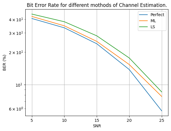
The following cell implements the evaluation pipeline as shown above. It runs the pipeline 3 times with perfect, ML, and LS channel estimation methods and prints the results at the end. As it can be seen, the ML-based channel estimation performs better than LS method which is based on interpolation.
[4]:
numFrames = 2                               # Number of time-domain frames
snrDbs = [5,10,15,20,25]                    # SNR values (in dB) for which we want to evaluate the model
freqDomain = False                          # Set to True to apply channel in frequency domain

carrier = Carrier(numRbs=51, spacing=30)    # Create a carrier with 51 RBs and 30KHz subcarrier spacing
bwp = carrier.curBwp                        # The only bandwidth part in the carrier

# Create a PDSCH object
pdsch = PDSCH(bwp, interleavingBundleSize=0, numLayers=2, nID=carrier.cellId, modulation="16QAM")
pdsch.setDMRS(prgSize=0, configType=2, additionalPos=2)     # Specify the DMRS configuration

numSlots = bwp.slotsPerFrame*numFrames                      # Total number of slots
results = {}                                                # Dictionary to save the results

for chanEstMethod in ["Perfect", "ML", "LS"]:               # Three different channel estimation methods
    results[chanEstMethod] = {}
    print("\nSimulating end-to-end for \"%s\", with \"%s\" channel estimation, in %s domain."%
          ("16QAM", chanEstMethod, "frequency" if freqDomain else "time"))
    print("SNR(dB)   Total Bits   Bit Errors   BER(%)   time(Sec.)")
    print("-------   ----------   ----------   ------   ----------")
    for snrDb in snrDbs:                                # For each SNR value in snrDbs
        random.setSeed(123)                             # Making the results reproducible for each SNR
        t0 = time.time()                                # Start time for each SNR
        carrier.slotNo = 0

        # Creating a CdlChannel object
        channel = CdlChannel('C', delaySpread=300, carrierFreq=4e9, dopplerShift=5,
                             txAntenna = AntennaPanel([2,2], polarization="x"),  # 8 TX antenna
                             rxAntenna = AntennaPanel([1,1], polarization="+"),  # 2 RX antenna
                             seed = 123,
                             timing = "nearest")

        bitErrors = 0
        totalBits = 0

        for slotNo in range(numSlots):
            grid = pdsch.getGrid()                      # Create a resource grid populated with DMRS
            numBits = pdsch.getBitSizes(grid)[0]        # Number of bits available in the resource grid
            txBits = random.bits(numBits)               # Create random binary data

            pdsch.populateGrid(grid, txBits)            # Map/modulate the data to the resource grid

            # Store the indexes of the PDSCH data in pdschIndexes to be used later.
            pdschIndexes = pdsch.getReIndexes(grid, "PDSCH")

            # Getting the Precoding Matrix, and precoding the resource grid
            channelMatrix = channel.getChannelMatrix(bwp)           # Get the channel matrix
            precoder = pdsch.getPrecodingMatrix(channelMatrix)      # Get the precoder matrix from PDSCH object
            precodedGrid = grid.precode(precoder)                   # Perform the precoding

            if freqDomain:
                rxGrid = precodedGrid.applyChannel(channelMatrix)   # Apply the channel in frequency domain
                rxGrid = rxGrid.addNoise(snrDb=snrDb)               # Add noise
            else:
                txWaveform = precodedGrid.ofdmModulate()            # OFDM Modulation
                maxDelay = channel.getMaxDelay()                    # Get the max. channel delay
                txWaveform = txWaveform.pad(maxDelay)               # Pad with zeros
                rxWaveform = channel.applyToSignal(txWaveform)      # Apply channel in time domain
                noisyRxWaveform = rxWaveform.addNoise(snrDb=snrDb, nFFT=bwp.nFFT)  # Add noise
                offset = channel.getTimingOffset()                  # Get timing info for synchronization
                syncedWaveform = noisyRxWaveform.sync(offset)       # Synchronization
                rxGrid = syncedWaveform.ofdmDemodulate(bwp)         # OFDM demodulation

            if chanEstMethod == "Perfect":                          # Perfect Channel Estimation
                estChannelMatrix = channelMatrix @ precoder[None,...]
            elif chanEstMethod == "LS":                             # LS + Interpolation Channel Estimation
                estChannelMatrix, noiseEst = rxGrid.estimateChannelLS(pdsch.dmrs, polarInt=False,
                                                                      kernel='linear')
            elif chanEstMethod == "ML":                             # ML-Based Channel Estimation
                estChannelMatrix = mlChanEst(pdsch.dmrs, rxGrid, model)
            else: assert(0)

            eqGrid, llrScales = rxGrid.equalize(estChannelMatrix)           # Equalization

            rxBits = pdsch.getHardBitsFromGrid(eqGrid, pdschIndexes)[0]     # Demodulation
            bitErrors += np.abs(rxBits-txBits).sum()                        # Calculating number of bit errors
            totalBits += numBits
            print("\r  %3d      %8d     %8d    %6.2f    %6.2f"%(snrDb, totalBits, bitErrors,
                                                                bitErrors*100/totalBits,time.time()-t0),end='')

            carrier.goNext()                        # Prepare the carrier object for the next slot
            channel.goNext()                        # Prepare the channel model for the next slot

        dt = time.time()-t0                         # Total time for this SNR
        results[chanEstMethod][snrDb] = {"totalBits":totalBits,
                                         "bitErrors":bitErrors,
                                         "BER":      bitErrors*100/totalBits,
                                         "Time":     dt}
        print("\r  %3d      %8d     %8d    %6.2f    %6.2f"%(snrDb, totalBits, bitErrors,
                                                        bitErrors*100/totalBits, dt))

# Compare the results in a plot:
for i,chanEstMethod in enumerate(['Perfect', 'ML', 'LS']):
    bers = [results[chanEstMethod][snrDb]["BER"] for snrDb in snrDbs]
    plt.plot(snrDbs, bers, label=chanEstMethod)
plt.legend()
plt.title("Bit Error Rate for different mothods of Channel Estimation.");
plt.grid()
plt.xlabel("SNR")
plt.xticks(snrDbs)
plt.ylabel("BER (%)")
plt.yscale('log')
plt.show()
Simulating end-to-end for "16QAM", with "Perfect" channel estimation, in time domain.
SNR(dB)   Total Bits   Bit Errors   BER(%)   time(Sec.)
-------   ----------   ----------   ------   ----------
    5       2545920      1036799     40.72     10.68
   10       2545920       850716     33.41     10.37
   15       2545920       606267     23.81     10.36
   20       2545920       350625     13.77     10.40
   25       2545920       145817      5.73     10.51

Simulating end-to-end for "16QAM", with "ML" channel estimation, in time domain.
SNR(dB)   Total Bits   Bit Errors   BER(%)   time(Sec.)
-------   ----------   ----------   ------   ----------
    5       2545920      1082460     42.52     10.93
   10       2545920       887201     34.85     10.81
   15       2545920       636788     25.01     10.74
   20       2545920       388967     15.28     10.62
   25       2545920       196876      7.73     10.67

Simulating end-to-end for "16QAM", with "LS" channel estimation, in time domain.
SNR(dB)   Total Bits   Bit Errors   BER(%)   time(Sec.)
-------   ----------   ----------   ------   ----------
    5       2545920      1138786     44.73     10.64
   10       2545920       968019     38.02     10.74
   15       2545920       717426     28.18     10.73
   20       2545920       448406     17.61     10.74
   25       2545920       217902      8.56     10.71
[ ]: