Beam Sweeping with Antenna Panels and Arrays

import numpy as np
import matplotlib.pyplot as plt
import matplotlib.animation as animation
from IPython.display import HTML, Markdown, display

from neoradium import AntennaElement, AntennaPanel, AntennaArray

A Linear Antenna Panel with Dual Polarization

# Create a linear antenna panel with 8 elements (4 antenna positions with dual polarization)
txAntenna=AntennaPanel([1,4], polarization='x')
# Get beam sweeping information:
precoders, beams = txAntenna.getSweepingBeams(numTheta=1, numPhi=8, polStrategy="equal")
# 'precoders' is a 'numPorts × numBeams' complex matrix.
numPorts, numBeams = precoders.shape
print(f"Number of ports: {numPorts}")
print(f"{len(beams[0])} Beams:")
print("  Beam    Theta     Phi     Pol")
print("  ----    -----    -----    ---")
for i in range(numBeams):
    print(f"   {i}     {np.round(beams[0][i],1):5.1f}     {np.round(beams[1][i],1):5.1f}     {beams[2][i]}")

Number of ports: 8
8 Beams:
  Beam    Theta     Phi     Pol
  ----    -----    -----    ---
   0      90.0     -60.0     x
   1      90.0     -38.2     x
   2      90.0     -21.8     x
   3      90.0      -7.1     x
   4      90.0       7.1     x
   5      90.0      21.8     x
   6      90.0      38.2     x
   7      90.0      60.0     x

# Draw beams (animation):
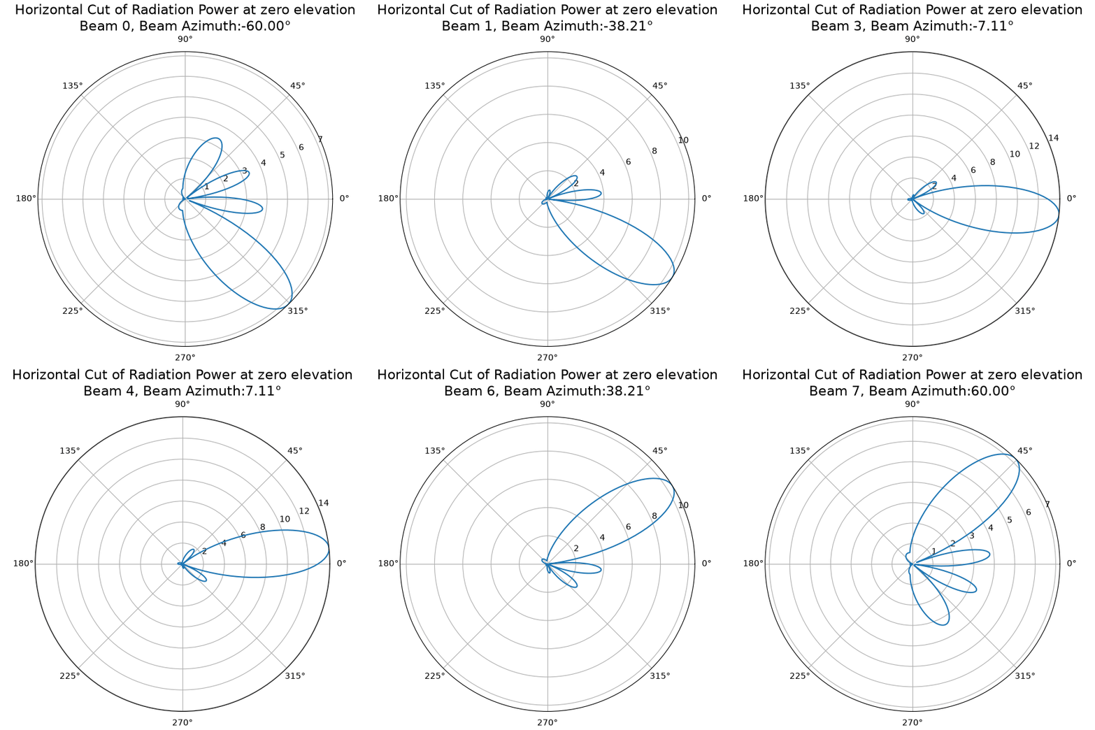
# Note: The ±60° beams are attenuated due to the element pattern (based on 38.901).
# To verify, try larger beamwidths or use an omnidirectional element.
# Also observe the power of different beams: they become weaker toward the extreme angles (-60° and +60°).
#
# A panel for a sector works best between -45° and +45°. UEs at the sector edges experience
# attenuated beams, which is consistent with practical deployments.
#
# Options to better cover the full 360°:
#   - Use multiple panels per sector
#   - Use 4 panels with 90° offsets (common in small cells, dense urban deployments, and FR2)

title = "Horizontal Cut of Radiation Power at zero elevation\nBeam %d, Beam Azimuth:%.2f°"
# Initial call to get a figure and axis for the animation:
ax = txAntenna.drawRadiation(theta=90, radiationType="Field", normalize=False, weights=precoders[:,0],
                             title = title%(0,beams[1][0]))
# Callback function to update the radiation pattern:
def updateCb(frame):
    ax.clear()
    i = frame % numBeams
    txAntenna.drawRadiation(theta=90, radiationType="Field", normalize=False, weights=precoders[:,i],
                            title = title%(i,beams[1][i]), ax=ax)
    return ()

# Create animation of beams:
fig = ax.get_figure()
anim = animation.FuncAnimation(fig, updateCb, frames = numBeams,  interval=1000, blit=False, repeat=False)
plt.close(fig)   # Prevent duplicate static plot

# Save the animation to a GIF file and show it below
anim.save("BeamSweep.gif", writer=animation.PillowWriter(fps=1))
display(Markdown("![demo](BeamSweep.gif)"))

# Another option is to use the following command, which gives you more control over
# running and pausing the animation.
# HTML(anim.to_jshtml())

A 4×4 Antenna Panel with Dual Polarization

# Create an antenna panel with 32 elements (16 antenna positions with dual polarization)
txAntenna=AntennaPanel([4,4], polarization='x')
# Get beam sweeping information:
precoders, beams = txAntenna.getSweepingBeams(numTheta=4, numPhi=4, thetaSpan=40, polStrategy="equal")
# 'precoders' is a 'numPorts × numBeams' complex matrix.
numPorts, numBeams = precoders.shape
print(f"Number of ports: {numPorts}")
print(f"{len(beams[0])} Beams:")
print("  Beam    Theta     Phi     Pol")
print("  ----    -----    -----    ---")
for i in range(numBeams):
    print(f"  {i:2d}     {np.round(beams[0][i],1):5.1f}     {np.round(beams[1][i],1):5.1f}     {beams[2][i]}")

Number of ports: 32
16 Beams:
  Beam    Theta     Phi     Pol
  ----    -----    -----    ---
   0      70.0     -60.0     x
   1      70.0     -16.8     x
   2      70.0      16.8     x
   3      70.0      60.0     x
   4      83.5     -60.0     x
   5      83.5     -16.8     x
   6      83.5      16.8     x
   7      83.5      60.0     x
   8      96.5     -60.0     x
   9      96.5     -16.8     x
  10      96.5      16.8     x
  11      96.5      60.0     x
  12     110.0     -60.0     x
  13     110.0     -16.8     x
  14     110.0      16.8     x
  15     110.0      60.0     x

# Initial call to obtain the figure and axis for the animation:
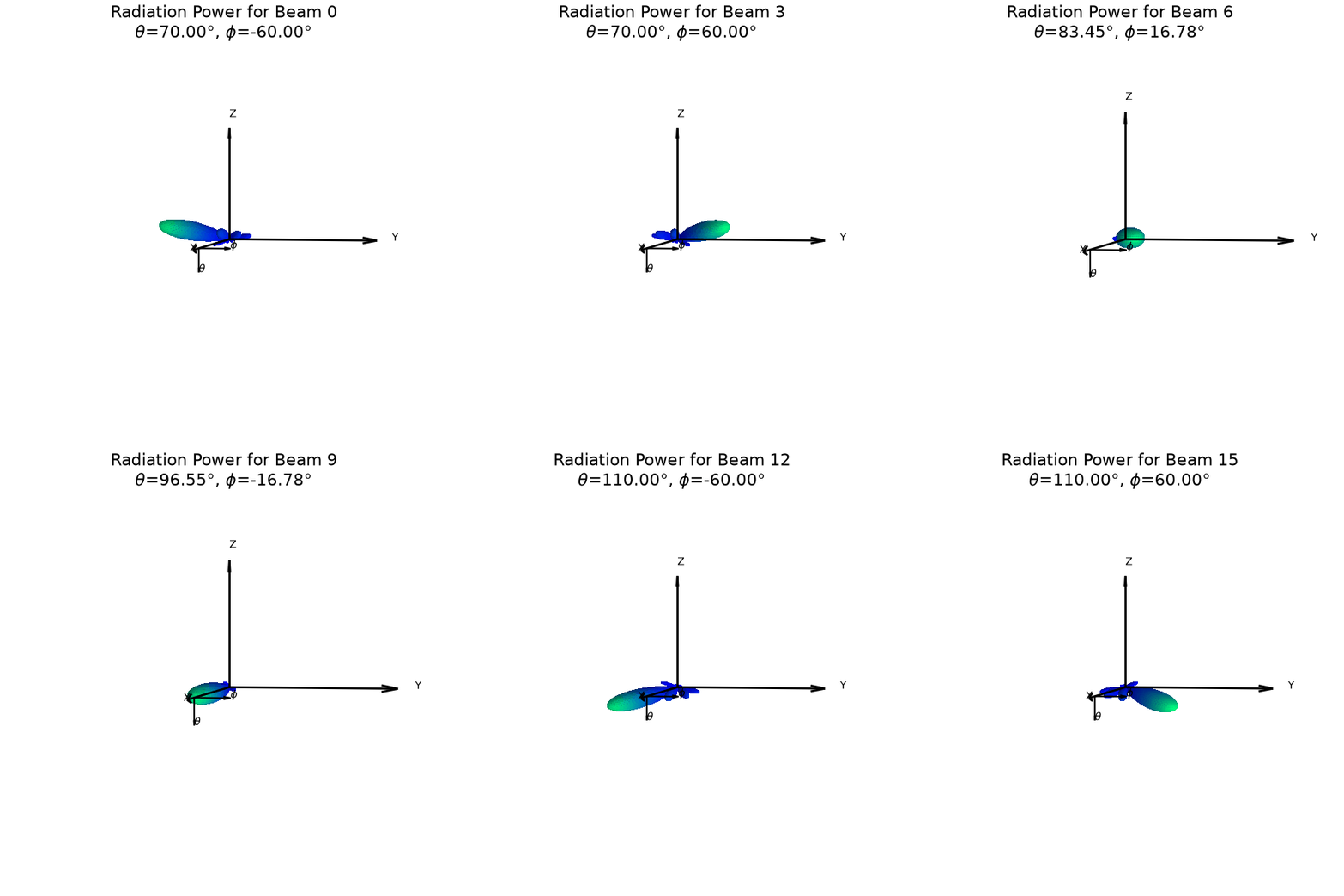
title = "Radiation Power for Beam %d\n$\\theta$=%.2f°, $\\phi$=%.2f°"
ax = txAntenna.drawRadiation(radiationType="Field", normalize=True, viewAngles=(10,3),
                             weights=precoders[:,0],
                             title = title%(0,beams[0][0],beams[1][0]))

# Callback function to update the radiation pattern:
def updateCb(frame):
    ax.clear()
    i = frame % numBeams
    print(f"\r  Now drawing beam {i} ...", end="")
    txAntenna.drawRadiation(radiationType="Field", normalize=True, viewAngles=(10,3),
                            weights=precoders[:,i],
                            title = title%(i,beams[0][i],beams[1][i]), ax=ax)
    ax.set_xlim(-1.5,1.5)
    ax.set_ylim(-1.5,1.5)
    ax.set_zlim(-1.5,1.5)
    if i==numBeams-1: print("\r  Done." + 50*" ")
    return ()

# Create animation of beams:
print("Preparing the animation:")
fig = ax.get_figure()
anim = animation.FuncAnimation(fig, updateCb, frames = numBeams,  interval=1000, blit=False, repeat=True)
plt.close(fig)      # Prevent duplicate static plot

# Save the animation to a GIF file and show it below
anim.save("BeamSweep3D.gif", writer=animation.PillowWriter(fps=1))
display(Markdown("![demo3d](BeamSweep3D.gif)"))

# Another option is to use the following command, which gives you more control over
# running and pausing the animation.
# HTML(anim.to_jshtml())

Preparing the animation:
  Done.

A Linear Antenna Array

# Now we create a 1×4 antenna array with four 2×2 panels. In this case, we have 8 antenna ports,
# and each port corresponds to one panel/polarization (e.g., 4 panels, 2 polarizations).
panelTemplate = AntennaPanel([2,2], polarization="x")
txArray = AntennaArray([1,4], panels=panelTemplate)

# Creating beam sweeping precoders for this array:
precoders, beams = txArray.getSweepingBeams(numTheta=1, numPhi=8, polStrategy="equal")

# 'precoders' is a 'numPorts × numBeams' complex matrix.
numPorts, numBeams = precoders.shape

print(f"Number of ports: {numPorts}")
print(f"precoders shape: {precoders.shape}")
print(f"{len(beams[0])} Beams:")
print("  Beam    Theta     Phi     Pol")
print("  ----    -----    -----    ---")
for i in range(numBeams):
    print(f"   {i}     {np.round(beams[0][i],1):5.1f}     {np.round(beams[1][i],1):5.1f}     {beams[2][i]}")

Number of ports: 8
precoders shape: (8, 8)
8 Beams:
  Beam    Theta     Phi     Pol
  ----    -----    -----    ---
   0      90.0     -60.0     x
   1      90.0     -38.2     x
   2      90.0     -21.8     x
   3      90.0      -7.1     x
   4      90.0       7.1     x
   5      90.0      21.8     x
   6      90.0      38.2     x
   7      90.0      60.0     x

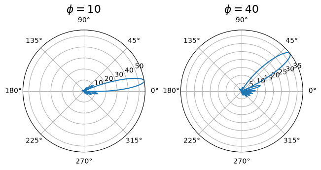
# Important note:
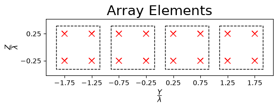
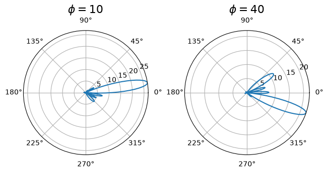
# This antenna array, with default internal precoders (B), behaves like a panel of 4 elements
# with 1λ spacing instead of 0.5λ. Since the spacing is larger than 0.5λ, grating lobes appear
# for some steering angles. This means we cannot reliably create beams at angles greater than 30°.

# Draw the antenna array:
txArray.showElements()

# Here is how two different beams look when using port-based precoding:
fig, ax = plt.subplots(1,2, layout='constrained', subplot_kw={'projection': 'polar'})
txArray.drawRadiation(theta=90, radiationType="Field", normalize=False, title = "$\\phi=10$",
                      weights=txArray.b @ txArray.getPortSteeringVector(90,10).flatten(), ax=ax[0])
txArray.drawRadiation(theta=90, radiationType="Field", normalize=False, title = "$\\phi=40$",
                      weights=txArray.b @ txArray.getPortSteeringVector(90,40).flatten(), ax=ax[1])

<PolarAxes: title={'center': '$\\phi=40$'}>

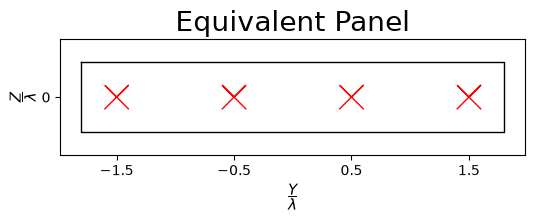
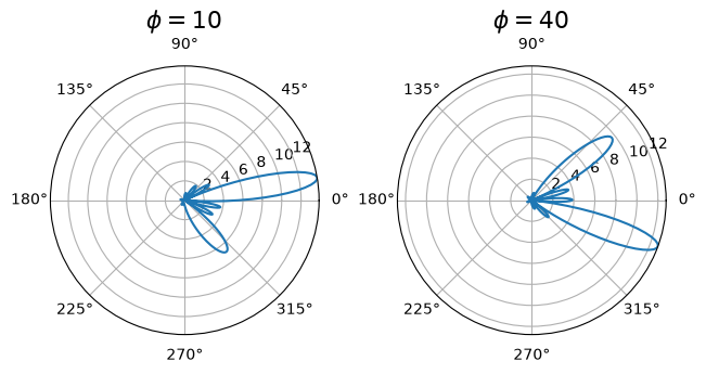
# To verify this, we can create a panel with 1λ spacing:
txPanel=AntennaPanel([1,4], polarization='x', spacing=(1,1))
txPanel.showElements(title="Equivalent Panel")

# Show the same two beams with this panel. As you can see the beams look very similar.
fig, ax = plt.subplots(1,2, layout='constrained', subplot_kw={'projection': 'polar'})
txPanel.drawRadiation(theta=90, radiationType="Field", normalize=False, title = "$\\phi=10$",
                      weights=txPanel.getPortSteeringVector(90,10).flatten(), ax=ax[0])
txPanel.drawRadiation(theta=90, radiationType="Field", normalize=False, title = "$\\phi=40$",
                      weights=txPanel.getPortSteeringVector(90,40).flatten(), ax=ax[1])

<PolarAxes: title={'center': '$\\phi=40$'}>

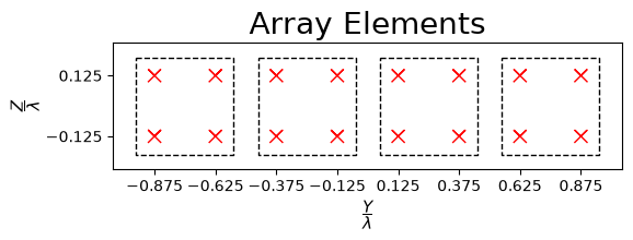
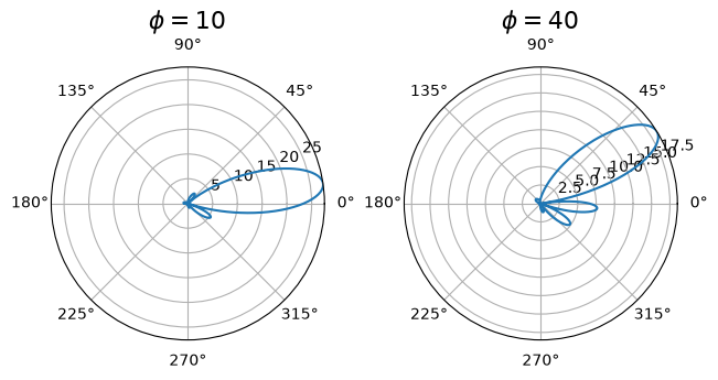
# One way to address this problem is to reduce the antenna spacing within each panel.
# For example, we use antenna panels with an internal spacing of 0.25λ. In this
# configuration, the panel centers are separated by 0.5λ, enabling the array to
# perform beamforming over larger angles.
panelTemplate = AntennaPanel([2,2], spacing=[0.25,0.25], polarization="x")
txArray = AntennaArray([1,4], panels=panelTemplate)

# Draw the antenna array:
txArray.showElements()

# Here is how two different beams look when using port-based precoding:
fig, ax = plt.subplots(1,2, layout='constrained', subplot_kw={'projection': 'polar'})
txArray.drawRadiation(theta=90, radiationType="Field", normalize=False, title = "$\\phi=10$",
                      weights=txArray.b @ txArray.getPortSteeringVector(90,10).flatten(), ax=ax[0])
txArray.drawRadiation(theta=90, radiationType="Field", normalize=False, title = "$\\phi=40$",
                      weights=txArray.b @ txArray.getPortSteeringVector(90,40).flatten(), ax=ax[1])

<PolarAxes: title={'center': '$\\phi=40$'}>

# Another option is to use element-based precoding, which enables beam steering over larger
# angles with narrower beams. This is because the element spacing remains 0.5λ, while the
# weights of individual elements can be controlled independently.

panelTemplate = AntennaPanel([2,2], polarization="x")
txArray = AntennaArray([1,4], panels=panelTemplate)

# Here is how the same beams look:
fig, ax = plt.subplots(1,2, layout='constrained', subplot_kw={'projection': 'polar'})
txArray.drawRadiation(theta=90, radiationType="Field", normalize=False, title = "$\\phi=10$",
                      weights=txArray.getSteeringVector(90,10).conj().flatten(), ax=ax[0])
txArray.drawRadiation(theta=90, radiationType="Field", normalize=False, title = "$\\phi=40$",
                      weights=txArray.getSteeringVector(90,40).conj().flatten(), ax=ax[1])

<PolarAxes: title={'center': '$\\phi=40$'}>