PDSCH end-to-end communication
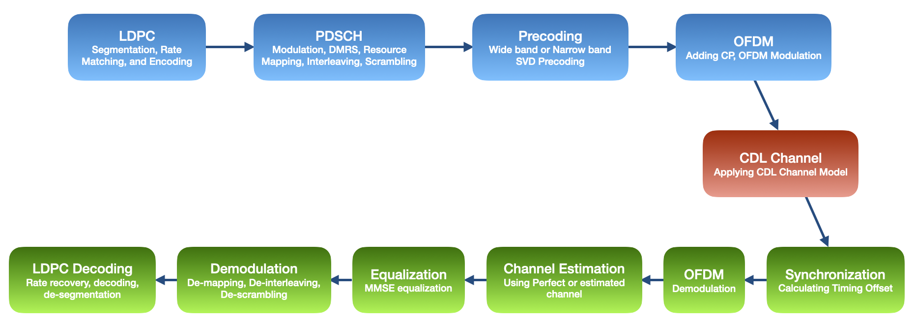
This notebook shows how an end-to-end communication through a 5G Physical Downlink Shared Channel (PDSCH) can be simulated in NeoRadium based on 3GPP NR standard. It demonstrates the following steps:
Creating LDPC encoder object, which performs transport block segmentation, LDPC encoding, and rate matching based on 3GPP TS 38.212.
Creating a
PDSCHobject and using it to populate a transmitted resource grid based on the encoded transport blocks. During this process, the PDSCH adds DMRS reference signals to the resource grid based on 3GPP TS 38.211 and TS 38.214.Creating a CDL channel model as specified in 3GPP TR 38.901 using the
CdlChannelclass. This class and the resource grid created by thePDSCH, are used to calculate a precoding matrix which is then used to precode the resource grid.Converting the precoded resource grid to a time-domain (transmitted) waveform through OFDM modulation performed by the
ofdmModulatemethod of theGridclass.Applying the CDL channel to the transmitted waveform to obtain the received waveform.
Synchronizing the received waveform by calculating the timing offset using the CdlChannel object.
Applying OFDM demodulation to the synchronized received waveform to get a received resource grid.
Estimating the channel matrix using the DMRS reference signals.
Equalizing the received resource grid using minimum mean-squared error (MMSE) equalization to cancel the effects of the communication channel.
Using the
getLLRsFromGridfunction ofPDSCHclass to extract log-likelihood ratios (LLRs) from the received resource grid.Performing rate-recovery and LDPC-decoding on the log-likelihood ratios.
Comparing the received bitstream with the original values used at the beginning of the pipeline.
Let’s get started by importing the NeoRadium modules used in the notebook.
[1]:
import numpy as np
import time

from neoradium import Carrier, PDSCH, CdlChannel, AntennaPanel, LdpcEncoder, Grid, random
Carrier Configuration
Here, using the Carrier class, we define a carrier with a 30 kHz subcarrier spacing and 51 resource blocks. The print function prints information about the carrier. Please note that by default a single bandwidth part is defined which covers the whole carrier. Additional bandwidth parts can be added to the carrier if needed.
[2]:
carrier = Carrier(numRbs=51, spacing=30)  # 51*12*30000 = 18,360,000 for 20 MHz Bandwidth
carrier.print()
bwp = carrier.curBwp                      # The only bandwidth part in the carrier
Carrier Properties:
  Cell Id:              1
  Bandwidth Parts:      1
  Active BWP:           0
  Bandwidth Part 0:
    Resource Blocks:    51 RBs starting at 0 (612 subcarriers)
    Subcarrier Spacing: 30 kHz
    CP Type:            normal
    Bandwidth:          18.36 MHz
    symbolsPerSlot:     14
    slotsPerSubFrame:   2
    nFFT:               1024
    frameNo:            0
    slotNo:             0
PDSCH and DMRS Configuration
Now let’s use the PDSCH class to configure the PDSCH communication parameters. Here we choose “Mapping Type A” and “QAM16” modulation (by default). We also set the number of layers to 2 and disable interleaving by setting interleavingBundleSize to zero.
Next, we set the DMRS configuration using the setDMRS method of the PDSCH class. Here we use DMRS configType set to 2 with 2 additional symbol time allocations (additionalPos=2). Although NeoRadium supports both wide band and narrow band precoding, we set the “Precoding RB Group (PRG)” size to 0, which means the same precoding is applied to all subcarriers (wideband precoding)
[3]:
pdsch = PDSCH(bwp, interleavingBundleSize=0, numLayers=2, nID=carrier.cellId)
pdsch.setDMRS(prgSize=0, configType=2, additionalPos=2)
pdsch.print()
PDSCH Properties:
  mappingType: A
  nID: 1
  rnti: 1
  numLayers: 2
  numCodewords: 1
  modulation: 16QAM
  portSet: [0, 1]
  symSet:   0   1   2   3   4   5   6   7   8   9  10  11  12  13
  prbSet:   0   1   2   3   4   5   6   7   8   9  10  11  12  13  14  15  16  17  18  19
           20  21  22  23  24  25  26  27  28  29  30  31  32  33  34  35  36  37  38  39
           40  41  42  43  44  45  46  47  48  49  50
  interleavingBundleSize: 0
  PRG Size: Wideband
  Bandwidth Part:
    Resource Blocks:    51 RBs starting at 0 (612 subcarriers)
    Subcarrier Spacing: 30 kHz
    CP Type:            normal
    Bandwidth:          18.36 MHz
    symbolsPerSlot:     14
    slotsPerSubFrame:   2
    nFFT:               1024
    frameNo:            0
    slotNo:             0
  DMRS:
    configType: 2
    nIDs: []
    scID: 0
    sameSeq: 1
    symbols: Single
    typeA1stPos: 2
    additionalPos: 2
    cdmGroups: [0, 0]
    deltaShifts: [0, 0]
    allCdmGroups: [0]
    symSet: [ 2  7 11]
    REs (before shift): [0, 1, 6, 7]
    epreRatioDb: 0 (dB)
Channel Coding Configuration
Now it’s time to define the parameters for LDPC channel coding. NeoRadium provides the LdpcEncoder and LdpcDecoder classes. These classes can be used to perform data segmentation and de-segmentation, rate matching and rate recovery, and encoding and decoding. Here we first set our desired code rate, then create an LdpcEncoder object that will be used for LDPC encoding.
[4]:
codeRate = 490/1024
ldpcEncoder = LdpcEncoder(baseGraphNo=1, modulation=pdsch.modems[0].modulation,
                          txLayers=pdsch.numLayers, targetRate=codeRate)
Resource Grid Creation and Mapping
Now that we have created the PDSCH and LDPC encoder objects, we can use them to perform channel coding and resource mapping. In the following cell, we first create a resource grid object using the getGrid method of the PDSCH object. This creates a resource grid, generates the DMRS reference signals, and places them in their specified locations within the grid.
The method getTxBlockSize is used to calculate the transport block size(s) based on the resources available in the grid for data transmission at the specified code rate. This function calculates the transport block size based on 3GPP TS 38.214.
Once we have the transport block size, we create random bits for transmission using the utility function makeRandomBits.
The function getBitSizes returns the total bit capacity of the resource grid for each codeword. This is the total number of encoded data bits that can be transmitted using the resource grid. It is used to perform rate-matching by the LdpcEncoder class.
The function getRateMatchedCodeBlocks performs segmentation, rate-matching, and LDPC encoding in a single call.
Once we have the rate-matched encoded bits, we can map them to the available resources in the resource grid. This is exactly what the populateGrid method of the PDSCH class does. This function first converts bits to complex symbols using the QAM modulation and then assigns the symbols to the available resource elements in the resource grid across different time, frequency, and layer locations.
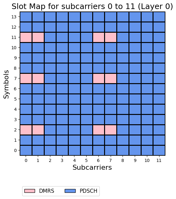
The drawMap method of the Grid class is used here to show the allocation of data and DMRS in the resource grid.
[5]:
random.setSeed(123)                          # Making the results reproducible.
grid = pdsch.getGrid()                       # Create a resource grid already populated with DMRS
txBlockSize = pdsch.getTxBlockSize(codeRate) # Calculate the Transport Block Size based on 3GPP TS 38.214
txBlock = random.bits(txBlockSize[0])        # Create random binary data

numBits = pdsch.getBitSizes(grid)            # Actual number of bits available in the resource grid

# Now perform the segmentation, rate-matching, and encoding in one call:
rateMatchedCodeBlocks = ldpcEncoder.getRateMatchedCodeBlocks(txBlock, numBits[0])

# Now populate the resource grid with coded data. This includes QAM modulation and resource mapping.
pdsch.populateGrid(grid, rateMatchedCodeBlocks)

# Store the indexes of the PDSCH data in pdschIndexes to be used later.
pdschIndexes = pdsch.getReIndexes(grid, "PDSCH")

print("TX Block Size:", txBlockSize[0])
print("Number of bits:", numBits[0])
print("Size of the rate-matched coded block:", rateMatchedCodeBlocks.shape[0])

# Get statistics about the grid resource allocation
gridStats = grid.getStats()
print("Grid Allocation Stats:")
for key, value in gridStats.items():
    print("  %s: %d"%(key, value))

# Draw the map of grid showing the data and DMRS in the first RB of the BWP.
grid.drawMap()
TX Block Size: 30216
Number of bits: 63648
Size of the rate-matched coded block: 63648
Grid Allocation Stats:
  GridSize: 17136
  DMRS: 1224
  PDSCH: 15912
Channel Simulation and Precoding
The next step in the pipeline is the precoding process. In practice the precoding information is extracted at the UE side (The receiver in this case) from the estimated channel. Since we are demonstrating only downlink communication here, we assume that the precoding matrix is somehow available.
To calculate the precoding matrix we first need to define the channel model. Here we use a CDL channel model as specified in 3GPP TR 38.901. The CdlChannel class is used to create a channel model object. Here we are using a CDL-C model which simulates NLOS communication. We use delay spread of 300 ns and a doppler shift of 5 Hz. We also use a small MIMO configuration with 8 transmit antennas and 2 receive antennas. The print function of the CdlChannel class can be used to show all
properties of the CDL channel model.
To calculate the precoding matrix, we first get the channel matrix from the CdlChannel object. The channel matrix is a 4-D complex tensor of size lxkx NrxNt. Where l, k, Nr, and Nt are the number of time symbols (14), the number of subcarriers (51x12=612), the number of receiver antenna (2), and the number of transmitter antenna (8) respectively.
Once we have the channel matrix, the getPrecodingMatrix method of the PDSCH class is called to calculate and return the precoding matrix.
To precode the resource grid, we simply call the precode method of the Grid class passing in the precoding matrix.
[6]:
# Creating a CdlChannel object:
f0 = 4e9  # Carrier Frequency
channel = CdlChannel(bwp, 'C', delaySpread=300, carrierFreq=f0, dopplerShift=5,
                     txAntenna = AntennaPanel([2,4], polarization="|"),  # 8 TX antenna
                     rxAntenna = AntennaPanel([1,2], polarization="|"))  # 2 RX antenna
# channel.print()                                       # Uncomment to print all channel information

# Getting the Precoding Matrix, and precoding the resource grid
channelMatrix = channel.getChannelMatrix()              # Get the channel matrix
precoder = pdsch.getPrecodingMatrix(channelMatrix)      # Get the precoder matrix from the PDSCH object
precodedGrid = grid.precode(precoder)                   # Perform the precoding

print("Shape of Channel Matrix:        ", channelMatrix.shape)
print("Shape of Resource Grid:         ", grid.shape)
print("Shape of Precoded Resource Grid:", precodedGrid.shape)
Shape of Channel Matrix:         (14, 612, 2, 8)
Shape of Resource Grid:          (2, 14, 612)
Shape of Precoded Resource Grid: (8, 14, 612)
OFDM Modulation
To transmit the precoded resource grid, it must first be transformed into the time domain. The method ofdmModulate of the Grid class converts the precoded grid into a set of time-domain waveforms for each transmit antenna. The output of the OFDM modulation is a Waveform class that contains the time-domain waveforms for each transmit antenna.
[7]:
txWaveform = precodedGrid.ofdmModulate()
# txWaveform contains the waveforms in time domain for each transmitter antenna
print("Shape of txWaveform:", txWaveform.shape)
Shape of txWaveform: (8, 15360)
Applying the channel model to the transmitted waveform
Now we need to pass the transmitted waveform through our CDL channel model. Because channel models typically delay signals, we append zeros to the end of the waveform to ensure the entire signal is captured at the channel output. The number of these zeros depend on the maximum channel delay that can be obtained using the getMaxDelay method of the CdlChannel class. The pad method of the Waveform class appends zeros to the end of waveform.
Now the channel model can be applied to the transmitted waveform to obtain the received waveform. This is exactly what the applyToSignal method of the CdlChannel class does. The output is another Waveform object containing the received waveform for each receiver antenna.
[8]:
# Need to append zeros to the end of signal based on the maximum channel filter delay
maxDelay = channel.getMaxDelay()
print("Max Channel Delay:  ", maxDelay)
txWaveform = txWaveform.pad(maxDelay)

# Applying channel to the transmitted signal
rxWaveform = channel.applyToSignal(txWaveform)
print("Shape of rxWaveform:", rxWaveform.shape)
Max Channel Delay:   87
Shape of rxWaveform: (2, 15447)
Adding Noise
We can use the addNoise method of the Waveform class to add AWGN to the received signal. Since we are adding the noise in the time-domain, we need to provide an instance of BandwidthPart object to extract FFT information.
Here, we calculate the noise power using the SNR value and the received signal power by setting useRxPower to True. Please refer to the documentation of addNoise for more information about the useRxPower argument.
[9]:
from neoradium.utils import toLinear
noisyRxWaveform = rxWaveform.addNoise(snrDb=20, bwp=bwp, useRxPower=False)
Synchronization and OFDM Demodulation
Because of multiple path delays involved in the channel model, we need to find the best starting point in the received waveform. This is usually done by finding the position of maximum correlation between the received signal and reference signals. The function getTimingOffset of the CdlChannel provides this “timing offset” which is the number of samples we need to skip from the beginning of the received waveform.
After synchronization, the waveform can be used for OFDM demodulation to obtain the received resource grid. The class method ofdmDemodulate creates a Grid class instance containing the noisy received resource grid.
[10]:
# Synchronization: Get the timing offset
offset = channel.getTimingOffset()
syncedWaveform = noisyRxWaveform.sync(offset)
print("Timing Offset:                  ", offset)

# OFDM Demodulation
noisyRxGrid = syncedWaveform.ofdmDemodulate(bwp)
print("Shape of received resource grid:", noisyRxGrid.shape)
Timing Offset:                   13
Shape of received resource grid: (2, 14, 612)
Applying channel in Frequency Domain
You can also use a shortcut method of applying the channel model to the transmitted grid directly without going to time domain.
The method applyChannel of the Grid class can be used to apply a channel matrix to a resource grid. For example:
# Applying the channel matrix to the precoded grid
rxGrid = precodedGrid.applyChannel(channelMatrix)
Channel Estimation
The input to the channel estimation process is the received resource grid and the known reference signals (in this case DMRS) and the output is the estimated channel. Note that in this case the estimated channel includes the precoding process. This is because the DMRS reference signals were inserted into the resource grid before precoding.
Perfect Channel Estimation
For perfect channel estimation, we need to apply precoding to the channel matrix. This can be done by a simple matrix multiplication as shown in the following cell.
Practical Channel Estimation
The method estimateChannelLS of the Grid class can be used to estimate the channel matrix. This method performs CDM averaging, least-squares channel estimation at pilot locations, and applying interpolation to get the whole channel matrix.
[11]:
# Perfect channel estimation (Applying the precoding to the channel matrix)
# estChannelMatrix = channel.getEffChannel(channelMatrix, precoder)

# Least-squares channel estimation
estChannelMatrix, _ = noisyRxGrid.estimateChannelLS(pdsch.dmrs, polarInt=True, kernel='linear')

print("Shape of estimated channel:", estChannelMatrix.shape)
Shape of estimated channel: (14, 612, 2, 2)
Equalization
Now that we have an estimate of the channel matrix, we can use it for equalization. The method equalize of the Grid class uses the Minimum mean-squared error (MMSE) equalization algorithm to mitigate the effects of the channel in the received resource grid.
It outputs a Grid object containing the equalized received resource grid and the LLR scaling values which is used later to scale the log-likelihood ratios from the demodulation process.
[12]:
eqGrid, llrScales = noisyRxGrid.equalize(estChannelMatrix)
print("Shape of equalized grid:", eqGrid.shape)
print("Shape of LLR Scales:    ", llrScales.shape)
Shape of equalized grid: (2, 14, 612)
Shape of LLR Scales:     (2, 14, 612)
Demodulation, De-mapping, Descrambling
The method getLLRsFromGrid of the PDSCH object performs demodulation, de-mapping, and descrambling of the received grid in one call. The output of this process is a set of log-likelihood ratios (LLRs) extracted from the received resource grid for the each codeword. Note that in this example there is only one codeword.
[13]:
llrs = pdsch.getLLRsFromGrid(eqGrid, pdschIndexes, llrScales)
print("Length of LLRs for the first codeword:", llrs[0].shape[0])
Length of LLRs for the first codeword: 63648
Rate Recovery and LDPC decoding
We are close to the end of the pipeline. We just need to decode the LLRs to the actual transport blocks. To do this, we need an LDPC decoder object. The method getDecoder of the LdpcEncoder class conveniently creates a decoder object matching the parameters of the encoder.
The function recoverRate of the LDPC decoder object can then be used to recover the rate of LDPC code blocks based on the transport block size. This is based on the procedure specified in 3GPP TS 38.212.
The rate-recovered coded blocks are then ready to be LDPC-decoded using the decode method of the LdpcDecoder class (Each coded block is decoded separately). The output is a set of the decoded blocks.
[14]:
# Create an LDPC Decoder object using the same parameters used to create the encoder.
ldpcDecoder = ldpcEncoder.getDecoder()

# Do rate recovery (Note: We have only one codeword in this example)
rxCodedBlocks = ldpcDecoder.recoverRate(llrs[0], txBlockSize[0])
print("Shape of rxCodedBlocks: ", rxCodedBlocks.shape)

# LDPC-Decoding
decodedBlocks = ldpcDecoder.decode(rxCodedBlocks, numIter=20)
print("Shape of Decoded Blocks:", decodedBlocks.shape)
Shape of rxCodedBlocks:  (4, 23232)
Shape of Decoded Blocks: (4, 7744)
CRC checking and De-segmentation
The CRC of each decoded block must be checked and then the decoded blocks need to be merged (de-segmented) to provide the transport blocks. The method checkCrcAndMerge of the LdpcDecoder class does exactly this. The output of this method is a decoded transport block which also contains a transport block CRC appended at the end.
The checkCrc method of the LdpcDecoder class can be used to check the transport block CRC.
[15]:
decodedTxBlockWithCRC, crcMatch = ldpcDecoder.checkCrcAndMerge(decodedBlocks)
print("Shape of decoded transport block:", decodedTxBlockWithCRC.shape)
print("CRC Match for each decoded block:", crcMatch)

txBlockCrcMatch = ldpcDecoder.checkCrc(decodedTxBlockWithCRC,'24A')
print("Transport block CRC Match:       ", txBlockCrcMatch)
Shape of decoded transport block: (30240,)
CRC Match for each decoded block: [ True  True  True  True]
Transport block CRC Match:        True
Comparing the decoded transport block with the original
We can get the decoded transport block by removing the 24-bit CRC at the end. Then, we can compare the results with the original transport block that was randomly generated at the beginning of this pipeline.
[16]:
decodedTxBlock = decodedTxBlockWithCRC[:-24]  # remove the transport block CRC
print("The number of bit mismatches between the decoded transport block and original:",np.abs(decodedTxBlock-txBlock).sum())
The number of bit mismatches between the decoded transport block and original: 0
[ ]:
[ ]: