NR PDSCH Throughput with HARQ
This notebook demonstrates how to measure the physical downlink shared channel (PDSCH) throughput of a 5G New Radio (NR) link, as specified in the 3GPP NR standard. It is similar to the MATLAB example NR PDSCH Throughput and showcases the use of the following NeoRadium features:
Carrier and Bandwidth Part classes.
PDSCH and DMRS objects.
LDPC and HARQ capabilities.
CDL channel model and extraction of channel matrix and precoding matrix.
Resource grids, populating them, and applying channel models to them.
[1]:
import numpy as np
import scipy.io
import time
import matplotlib.pyplot as plt

from neoradium import Carrier, PDSCH, CdlChannel, AntennaPanel, LdpcEncoder, random, HarqEntity, SnrScheduler
[2]:
# Create a Carrier object with 51 resource blocks and 30KHz subcarrier spacing
carrier = Carrier(numRbs=51, spacing=30)
carrier.print()
bwp = carrier.curBwp                      # The only bandwidth part in the carrier
Carrier Properties:
  Cell Id:              1
  Bandwidth Parts:      1
  Active BWP:           0
  Bandwidth Part 0:
    Resource Blocks:    51 RBs starting at 0 (612 subcarriers)
    Subcarrier Spacing: 30 kHz
    CP Type:            normal
    Bandwidth:          18.36 MHz
    symbolsPerSlot:     14
    slotsPerSubFrame:   2
    nFFT:               1024
    frameNo:            0
    slotNo:             0
[3]:
# Initialize the modulation and code rate.
modulation = '16QAM'
codeRate = 490/1024

# Create a PDSCH onject with 2 tramsmission layers
pdsch = PDSCH(bwp, interleavingBundleSize=0, numLayers=2, nID=carrier.cellId)
pdsch.setDMRS(prgSize=0, configType=2, additionalPos=2, otherCdmGroups=[])
pdsch.print()

# Create an LDPC encoder object using base graph 1 and passing modulation and code rate settings
ldpcEncoder = LdpcEncoder(baseGraphNo=1,  modulation=modulation, txLayers=pdsch.numLayers, targetRate=codeRate)

# HARQ configuration:
harqType = "IR"                                     # "IR" -> "Incremental Redundancy", "CC" -> "Chase Combining"
numProc = 16                                        # Number of HARQ processes
harq = HarqEntity(ldpcEncoder, harqType, numProc)   # Create the HARQ entity
harq.print()

# Create the CDL channel model
channel = CdlChannel(bwp, 'C', delaySpread=300, carrierFreq=4e9, dopplerShift=5,
                     txAntenna = AntennaPanel([1,4], polarization="x"),                         # 8 TX antenna
                     rxAntenna = AntennaPanel([1,1], polarization="+", beamWidth=[75,360]),     # 2 RX antenna, Omni-directional
                     rxOrientation = [0,0,0])                                                   # Default is [180,0,0]
print(channel)
PDSCH Properties:
  mappingType: A
  nID: 1
  rnti: 1
  numLayers: 2
  numCodewords: 1
  modulation: 16QAM
  portSet: [0, 1]
  symSet:   0   1   2   3   4   5   6   7   8   9  10  11  12  13
  prbSet:   0   1   2   3   4   5   6   7   8   9  10  11  12  13  14  15  16  17  18  19
           20  21  22  23  24  25  26  27  28  29  30  31  32  33  34  35  36  37  38  39
           40  41  42  43  44  45  46  47  48  49  50
  interleavingBundleSize: 0
  PRG Size: Wideband
  Bandwidth Part:
    Resource Blocks:    51 RBs starting at 0 (612 subcarriers)
    Subcarrier Spacing: 30 kHz
    CP Type:            normal
    Bandwidth:          18.36 MHz
    symbolsPerSlot:     14
    slotsPerSubFrame:   2
    nFFT:               1024
    frameNo:            0
    slotNo:             0
  DMRS:
    configType: 2
    nIDs: []
    scID: 0
    sameSeq: 1
    symbols: Single
    typeA1stPos: 2
    additionalPos: 2
    cdmGroups: [0, 0]
    deltaShifts: [0, 0]
    allCdmGroups: [0]
    symSet: [ 2  7 11]
    REs (before shift): [0, 1, 6, 7]
    epreRatioDb: 0 (dB)


HARQ Entity Properties:
  HARQ Type:            IR
  Num. Processes:       16
  Num. Codewords:       1
  RV sequence:          [0, 2, 3, 1]
  maxTries:             4
  Encoder:
    Base Graph:         1
    Modulation:         16QAM
    Number of layers:   2
    Target Rate:        0.478515625
  Decoder:
    Base Graph:         1
    Modulation:         16QAM
    Number of layers:   2


CDL-C Channel Properties:
  carrierFreq:          4 GHz
  normalizeGains:       True
  normalizeOutput:      True
  txDir:                Downlink
  filterLen:            16 samples
  delayQuantSize:       64
  stopBandAtten:        80 dB
  dopplerShift:         5 Hz
  coherenceTime:        84.628 milliseconds
  delaySpread:          300 ns
  ueDirAZ:              0.0°, 90.0°
  Cross Pol. Power:     7 dB
  angleSpreads:         2° 15° 3° 7°
  TX Antenna:
    Total Elements:     8
    spacing:            0.5𝜆, 0.5𝜆
    shape:              1 rows x 4 columns
    polarization:       x
  RX Antenna:
    Total Elements:     2
    spacing:            0.5𝜆, 0.5𝜆
    shape:              1 rows x 1 columns
    polarization:       +
  hasLOS:               False
  NLOS Paths (24):
    Delays (ns):        0.000 62.97 66.57 69.87 65.28 190.9 193.4 196.8 197.5 238.0 246.3 280.0
                        368.5 392.4 651.1 813.1 1277. 1380. 1647. 1682. 1891. 1991. 2112. 2595.
    Powers (dB):        -4.40 -1.20 -3.50 -5.20 -2.50 0.000 -2.20 -3.90 -7.40 -7.10 -10.7 -11.1
                        -5.10 -6.80 -8.70 -13.2 -13.9 -13.9 -15.8 -17.1 -16.0 -15.7 -21.6 -22.8
    AODs (Deg):         -47  -23  -23  -23  -41  0    0    0    73   -64  80   -97
                        -55  -64  -78  103  99   89   -102 92   93   107  119  -124
    AOAs (Deg):         -101 120  120  120  -128 170  170  170  55   66   -48  47
                        68   -69  82   31   -16  4    -14  10   6    1    -22  34
    ZODs (Deg):         97   99   99   99   101  99   99   99   105  95   106  94
                        104  104  93   104  95   93   92   107  93   93   105  108
    ZOAs (Deg):         88   72   72   72   70   75   75   75   67   64   71   60
                        91   60   61   101  62   67   53   62   52   62   58   57
[4]:
# Print header lines:
print("SNR(dB)  Tx Bits     Rx Bits     Throughput(%)  TX Blocks  RX Blocks  BLER(%)  Retry Mean  time(Sec.)")
print("-------  ----------  ----------  -------------  ---------  ---------  -------  ----------  ----------")

snrScheduler = SnrScheduler(6,1, loSnrVal=0, hiSnrVal=100)      # Start at 6 dB, use increments of 0.2 dB
numSlots = 1000                                                 # The number of slots transmitted for each SNR value
for snrDb in snrScheduler:
    random.setSeed(123)
    channel.restart()                                           # Reset the channel and the bandwidth part associated with it
    harq.reset()                                                # Reset HARQ state and buffers

    t0 = time.time()                                            # Start the timer
    for s in range(numSlots):                                   # The inner loop doing 'numSlot' transmissions
        grid = bwp.createGrid(pdsch.numLayers)                  # Create a resource grid with 2 layers
        pdsch.allocateResources(grid)                           # Allocat PDSCH resources including DMRS
        txBlockSizes = pdsch.getTxBlockSize(codeRate)           # Calculate the Transport Block Size (TBS)
        numBits = pdsch.getBitSizes(grid)                       # Total number of PDSCH data bits available in the resource grid

        # Preparing the transport blocks
        txBlocks = []                                           # Transport blocks, one per codeword.
        for c in range(harq.numCW):
            if harq.needNewData[c]:                             # New transmission.
                txBlocks += [ random.bits(txBlockSizes[c]) ]    # Create random bits for new transmissions
            else:                                               # Retransmission
                txBlocks += [ None ]                            # Set transport block to None to indicate a retransmission

        # The following function returns a coded, rate-matched bitstream, ready for transmission/retransmission
        rateMatchedCodeBlocks = harq.getRateMatchedCodeBlocks(txBlocks, numBits)

        pdsch.populateGrid(grid, rateMatchedCodeBlocks)         # Map/modulate the data to the resource grid

        channelMatrix = channel.getChannelMatrix()              # Get channel matrix (Assuming perfect channel estimation)
        precoder = pdsch.getPrecodingMatrix(channelMatrix)      # Get precoding matrix based on the channel matrix

        precodedGrid = grid.precode(precoder)                   # Perform precoding

        rxGrid = precodedGrid.applyChannel(channelMatrix)       # Apply the channel to the precoded resource (Freq. domain)
        noisyRxGrid = rxGrid.addNoise(snrDb=snrDb, useRxPower=True) # Add noise (Using RX power to calcualte Noise Power)

        # Calculate the effective channel matrix with the precoding effect. This is assuming perfect channel
        # estimation. For practical channel estimation we can use the DMRS reference signals and use the
        # "estimateChannelLS" method of resource grid object.
        effChannelMatrix = channel.getEffChannel(channelMatrix, precoder)

        # Use the effective channel matrix to equalize the received resource grid
        eqGrid, llrScales = noisyRxGrid.equalize(effChannelMatrix)

        # Demodulate the equalized resource grid (eqGrid) to get the Log-Likelihood values
        llrs = pdsch.getLLRsFromGrid(eqGrid, pdsch.dataIndices, llrScales)

        # Use HARQ entity to decode the LLRs to transport blocks
        decodedTxBlocks, blockErrors = harq.decodeLLRs(llrs, txBlockSizes, numIter=2)

        # Get the statistics from HARQ entity and print them:
        print("\r%-7d  %-10d  %-10d  %-13.2f  %-9d  %-9d  %-7.2f  %-10.2f  %-10.2f"
              %(snrDb, harq.totalTxBits, harq.totalRxBits, harq.throughput, harq.totalTxBlocks,
                harq.totalRxBlocks, harq.bler, harq.meanTries, time.time()-t0), end='')

        channel.goNext()
        harq.goNext()

    snrScheduler.setData(harq.throughput)
    print("")
SNR(dB)  Tx Bits     Rx Bits     Throughput(%)  TX Blocks  RX Blocks  BLER(%)  Retry Mean  time(Sec.)
-------  ----------  ----------  -------------  ---------  ---------  -------  ----------  ----------
6        30216000    3263328     10.80          1000       108        89.20    3.48        141.18
5        30216000    1057560     3.50           1000       35         96.50    3.85        140.29
4        30216000    0           0.00           1000       0          100.00   4.00        140.27
3        30216000    0           0.00           1000       0          100.00   4.00        141.62
7        30216000    4774128     15.80          1000       158        84.20    3.04        144.14
8        30216000    6164064     20.40          1000       204        79.60    2.62        147.26
9        30216000    8067672     26.70          1000       267        73.30    2.08        152.38
10       30216000    9971280     33.00          1000       330        67.00    1.71        156.90
11       30216000    11059056    36.60          1000       366        63.40    1.53        161.82
12       30216000    13627416    45.10          1000       451        54.90    1.15        166.98
13       30216000    18129600    60.00          1000       600        40.00    0.66        180.91
14       30216000    21544008    71.30          1000       713        28.70    0.40        196.69
15       30216000    23296536    77.10          1000       771        22.90    0.30        207.68
16       30216000    24716688    81.80          1000       818        18.20    0.22        211.19
17       30216000    25472088    84.30          1000       843        15.70    0.19        212.86
18       30216000    26499432    87.70          1000       877        12.30    0.14        219.43
19       30216000    27375696    90.60          1000       906        9.40     0.10        220.38
20       30216000    28433256    94.10          1000       941        5.90     0.06        225.19
21       30216000    29672112    98.20          1000       982        1.80     0.02        230.49
22       30216000    30185784    99.90          1000       999        0.10     0.00        232.16
23       30216000    30216000    100.00         1000       1000       0.00     0.00        232.53
24       30216000    30216000    100.00         1000       1000       0.00     0.00        229.08
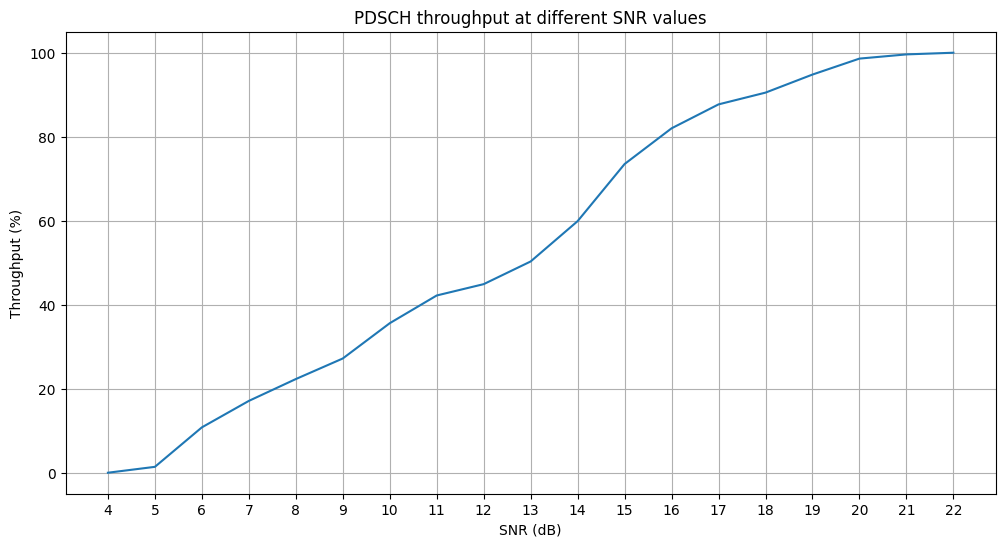
[5]:
# Draw the throughput graph:
snrDbs, throughputs = snrScheduler.getSnrsAndData()
plt.figure(figsize=(12, 6))
plt.plot(snrDbs, throughputs)
plt.title("PDSCH throughput at different SNR values");
plt.grid()
plt.xlabel("SNR (dB)")
plt.xticks(snrDbs)
plt.ylabel("Throughput (%)")
plt.show()
[ ]: